[프로젝트] Scene graph to Video generation with diffusion model - (1) 개념정리
Inha univ. Scene Graph를 Condition으로 받는 video generation diffusion model 개발 \
SGDiff
Diffusion-Based Scene Graph to Image Generation with Masked Contrastive Pre-Training
기존에는 Scene Graph를 통해 layout을 예측하고 이를 가지고 image를 generation 하는 방법이 일반적으로 사용되었다.
이 논문은 clip이 사용하는 방법(image vector - text vextor)대로 기존에 pretrain된 VIT를 통해 얻은 벡터와 GCN으로 뽑은 graph vector를 동일하게 맞추는 작업 (이미지 간의 정렬)
논문에서는 SG encoder라 명명
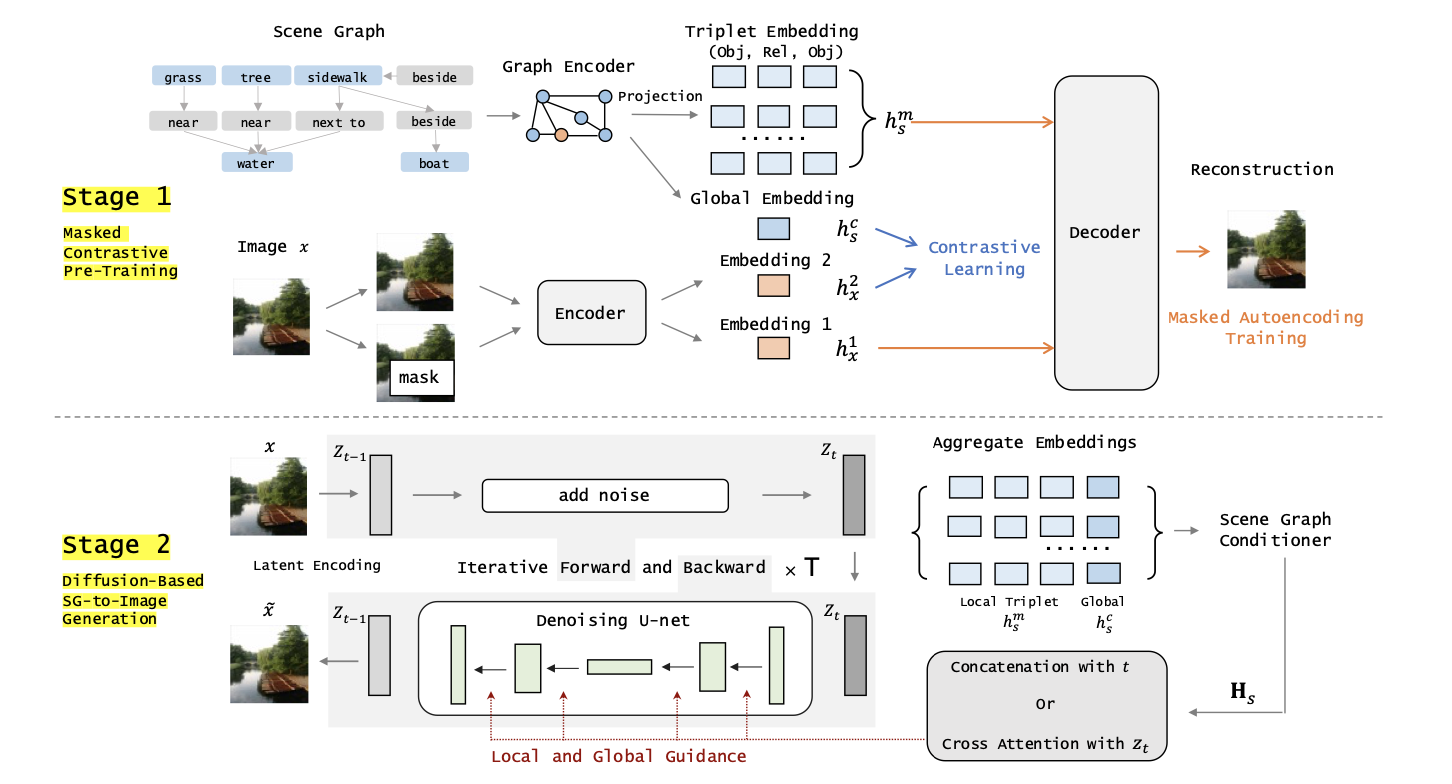
self-supervised learning : Loss는 contrastive, masked autoencoding를 사용
- contrastive : 두 global vector 비교 (InfoNCE)
- masked autoencoding : 두 local vector 비교
local embedding : 최종 출력 나오기 이전 Layer
global embedding : 최종 출력
두 loss는 약 10배 차이
diffusion model에 conditioning 방법으로 Cross-Attention 사용
dataset : Visual Genome, COCO-Stuff
graph encoding
def encode_graph_local_global(self, img, graph):
    batch_size, _, H, W = img.shape

    objs, boxes, triples, obj_to_img, triples_to_img = graph
    s, p, o = triples.chunk(3, dim=1)
    s, p, o = [x.squeeze(1) for x in [s, p, o]]
    edges = torch.stack([s, o], dim=1)

    obj_vecs = self.obj_embeddings(objs)
    pred_vecs = self.pred_embeddings(p)

    if isinstance(self.graph_conv, nn.Linear):
        obj_vecs = self.graph_conv(obj_vecs)
    else:
        obj_vecs, pred_vecs = self.graph_conv(obj_vecs, pred_vecs, edges)
    if self.graph_net is not None:
        obj_vecs, pred_vecs = self.graph_net(obj_vecs, pred_vecs, edges)

    # Global Branch
    obj_fea = self.pool_samples(obj_vecs, obj_to_img)
    pred_fea = self.pool_samples(pred_vecs, triples_to_img)
    graph_global_fea = self.graph_projection(torch.cat([obj_fea, pred_fea], dim=1))

    # Local Branch
    s_obj_vec, o_obj_vec = obj_vecs[s], obj_vecs[o]
    triple_vec = torch.cat([s_obj_vec, pred_vecs, o_obj_vec], dim=1)
    graph_local_fea = create_tensor_by_assign_samples_to_img(samples=triple_vec, sample_to_img=triples_to_img,
                                                            max_sample_per_img=self.max_sample_per_img,
                                                            batch_size=batch_size)

    return graph_local_fea, graph_global_fea
cross attention
def forward(self, x, context=None, mask=None):
    h = self.heads

    q = self.to_q(x)
    context = default(context, x)
    k = self.to_k(context)
    v = self.to_v(context)

    q, k, v = map(lambda t: rearrange(t, 'b n (h d) -> (b h) n d', h=h), (q, k, v))

    sim = einsum('b i d, b j d -> b i j', q, k) * self.scale

    if exists(mask):
        mask = rearrange(mask, 'b ... -> b (...)')
        max_neg_value = -torch.finfo(sim.dtype).max
        mask = repeat(mask, 'b j -> (b h) () j', h=h)
        sim.masked_fill_(~mask, max_neg_value)

    # attention, what we cannot get enough of
    attn = sim.softmax(dim=-1)

    out = einsum('b i j, b j d -> b i d', attn, v)
    out = rearrange(out, '(b h) n d -> b n (h d)', h=h)
    return self.to_out(out)
GCN (graph convolution network)
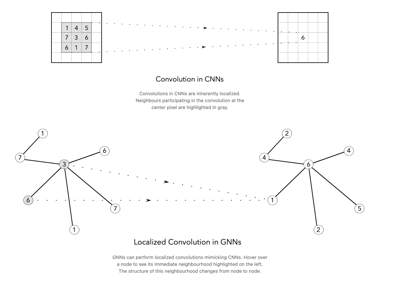
image에서의 CNN은 위치가 2차원 평면에 고정되어있기 때문에 kernel의 크기에 맞춰 범위 및 연산을 이해하기 쉽다.
Spatial GCN:
GCN 또한 이처럼 특정 노드에서 시작해 size 만큼 connection을 지나는 개수로 생각하면 쉽게 이해할 수 있다.
노드의 이웃에 대해 직접적으로 연산을 수행하여 각 노드의 특징을 학습
그래프 구조가 변해도 이웃 노드 간 관계만 업데이트 → 효율 좋음
spectral GCN:
spectrum : 이미지나 음성 데이터에서 eigenvalues로 측정한 양자들의 집합을 얻기위해 푸리에 해석(Fourier analysis) 과 같이 분해의 개념
-
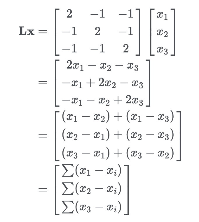
Laplacian operator : divergence of gradient, 벡터장(vector field)이 균일하지 않은 정도를 파악할 수 있는 방법 , 어떤 물체의 경계선 같은 곳에서 값이 높게 나옴
graph에서 Laplacian operator를 적용하면 각 노드와 이웃 노드 간의 차이를 나타냄
eigen decomposition
\[L=UΛU^T\]Laplacian의 eigenvalue는 Fourier transform의 spectrum 또는 frequency를 나타냄
-
Fourier Transform
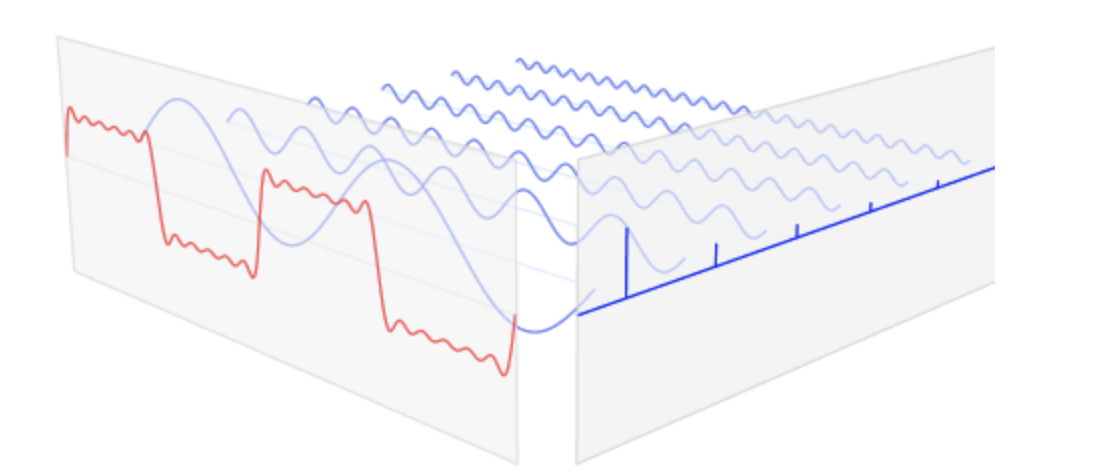
Fourier Transform
\[F(\omega) = \int_{-\infty}^{\infty} f(t) \cdot e^{-j\omega t} \, dt\]Inverse Fourier Transform
\[f(t) = \frac{1}{2\pi} \int_{-\infty}^{\infty} F(\omega) \cdot e^{j\omega t} \, d\omega\]
-
Convolution operator
\[(f * g)(t) = \int_{-\infty}^{\infty} f(\tau) \cdot g(t - \tau) \, d\tau\]
-
Convolution Theorem
Convolution 연산은 Fourier transform으로 대체 가능하다
\[\mathcal{F}\{f(t) * g(t)\} = F(\omega) \cdot G(\omega)\]시간 영역에서의 컨벌루션은 주파수 영역에서의 곱셈으로 변환
\[\mathcal{F}^{-1}\{F(\omega) * G(\omega)\} = f(t) \cdot g(t)\]곱과 convolution연산의 변환
\[h(t) = f(t) * g(t) = \mathcal{F}^{-1}\{F(\omega) \cdot G(\omega)\}\]
다음 convolution thorem은 CNN으로 아래와 같이 구현
\[Y(i, j) = \sum_{c=1}^{C} \sum_{m=1}^{k} \sum_{n=1}^{k} X(i + m - 1, j + n - 1, c) \cdot W(m, n, c)\]- 컨벌루션 계층 (Convolutional Layer) → convolution thorem
- 활성화 함수 (Activation Function)
- 풀링 계층 (Pooling Layer)
- 완전 연결 계층 (Fully Connected Layer)
code
def forward(self, obj_vecs, pred_vecs, edges):
    dtype, device = obj_vecs.dtype, obj_vecs.device
    O, T = obj_vecs.size(0), pred_vecs.size(0)
    Din, H, Dout = self.input_dim, self.hidden_dim, self.output_dim

    s_idx = edges[:, 0].contiguous()
    o_idx = edges[:, 1].contiguous()

    cur_s_vecs = obj_vecs[s_idx]
    cur_o_vecs = obj_vecs[o_idx]

    cur_t_vecs = torch.cat([cur_s_vecs, pred_vecs, cur_o_vecs], dim=1)
    new_t_vecs = self.net1(cur_t_vecs)

    new_s_vecs = new_t_vecs[:, :H]
    new_p_vecs = new_t_vecs[:, H:(H + Dout)]
    new_o_vecs = new_t_vecs[:, (H + Dout):(2 * H + Dout)]

    pooled_obj_vecs = torch.zeros(O, H, dtype=dtype, device=device)

    s_idx_exp = s_idx.view(-1, 1).expand_as(new_s_vecs)
    o_idx_exp = o_idx.view(-1, 1).expand_as(new_o_vecs)
    pooled_obj_vecs = pooled_obj_vecs.scatter_add(0, s_idx_exp, new_s_vecs)
    pooled_obj_vecs = pooled_obj_vecs.scatter_add(0, o_idx_exp, new_o_vecs)

    if self.pooling == 'avg':
        obj_counts = torch.zeros(O, dtype=dtype, device=device)
        ones = torch.ones(T, dtype=dtype, device=device)
        obj_counts = obj_counts.scatter_add(0, s_idx, ones)
        obj_counts = obj_counts.scatter_add(0, o_idx, ones)

        obj_counts = obj_counts.clamp(min=1)
        pooled_obj_vecs = pooled_obj_vecs / obj_counts.view(-1, 1)

    new_obj_vecs = self.net2(pooled_obj_vecs)

    return new_obj_vecs, new_p_vecs
Self-Supervised Learning
사람이 직접 레이블을 붙이지 않고도 모델이 데이터를 이해하도록 학습하는 머신 러닝 방식
보통 데이터의 일부를 이용해 다른 일부를 예측하도록 모델을 설정
- Autoregressive generation : next 예측
- Masked generation : masking된 부분 예측
- Innate relationship prediction : segmentation이나 rotation등의 transformation 본질은 동일
- Hybrid self-prediction : 앞선 방법들 결합
여기서는 Image와 Graph vector를 contrastive loss를 통해 일치시키는 과정과 특정 node에 해당하는 Image 부분을 mask 한 후 차이를 학습하는 과정 사용
contrastive learning : batch내의 data sample들 사이의 관계를 예측하는 task / positive, negative pair
- Triplet loss : distance를 기반하는 loss, embedding space에서의 sample 유사도, positive는 가깝게, negative는 멀게
-
InfoNCE : noise를 multiple로 확장한 loss,
\[\mathcal{L}_{\text{InfoNCE}} = - \log \frac{\exp(\text{sim}(\mathbf{z}_i, \mathbf{z}_i^+) / \tau)}{\sum_{j=1}^N \exp(\text{sim}(\mathbf{z}_i, \mathbf{z}_j) / \tau)}\]- \(z_i\)는 anchor(기준점)의 임베딩 벡터,
- \(z_i^+\)는 positive example의 임베딩 벡터,
- \(z_j\)는 모든 example(positive + negative)들의 임베딩 벡터,
- \(sim(⋅,⋅)\)은 두 벡터 간의 유사도, 일반적으로 코사인 유사도가 사용
- τ는 temperature , 유사도 값을 조정하여 모델이 더 세밀하게 학습할 수 있도록 함
- N은 positive example와 negative example를 포함한 총 샘플의 개수
보면 positive는 분자, negative는 분모에 있음 → anchor \(z_i\)의 가깝게, \(z _j\)는 anchor와 멀어지도록 학습
code
def forward(self, image_features, graph_features, logit_scale):
    device = image_features.device

    logits_per_image = logit_scale * image_features @ graph_features.T
    logits_per_graph = logit_scale * graph_features @ image_features.T

    num_logits = logits_per_image.shape[0]
    if self.prev_num_logits != num_logits or device not in self.labels:
        labels = torch.arange(num_logits, device=device, dtype=torch.long)
    else:
        labels = self.labels[device]

    total_loss = (
        F.cross_entropy(logits_per_image, labels) +
        F.cross_entropy(logits_per_graph, labels)
        ) / 2
  return total_loss