[논문분석] High-Resolution Image Synthesis with Latent Diffusion Models

Image generation with diffusion에 발전에 큰 기여을 한 오픈 소스 모델
[Page, Paper, Code]
LMU Munich, IWR, Heidelberg University, Runway CVPR 2022 (ORAL)

Abstract

By decomposing the image formation process into a sequential application of denoising autoencoders, diffusion models (DMs) achieve state-of-the-art synthesis results on image data and beyond. Additionally, their formulation allows for a guiding mechanism to control the image generation process without retraining. However, since these models typically operate directly in pixel space, optimization of powerful DMs often consumes hundreds of GPU days and inference is expensive due to sequential evaluations. To enable DM training on limited computational resources while retaining their quality and flexibility, we apply them in the latent space of powerful pretrained autoencoders. In contrast to previous work, training diffusion models on such a representation allows for the first time to reach a near-optimal point between complexity reduction and detail preservation, greatly boosting visual fidelity. By introducing cross-attention layers into the model architecture, we turn diffusion models into powerful and flexible generators for general conditioning inputs such as text or bounding boxes and high-resolution synthesis becomes possible in a convolutional manner. Our latent diffusion models (LDMs) achieve new state-of-the-art scores for image impainting and class-conditional image synthesis and highly competitive performance on various tasks, including text-to-image synthesis, unconditional image generation and super-resolution, while significantly reducing computational requirements compared to pixel-based DMs.

diffusion model 은 이미지 생성에서 뛰어남

픽셀 공간에서 동작하는 diffusion model은 최적화하는 데 비용이 많이 듬

latent space에서 동작하여, 품질과 유연성을 유지하면서 제한된 컴퓨팅 리소스 활용

오토인코더의 잠재 공간에 적용

복잡성 감소와 디테일 보존 사이의 최적점에 도달

모델 아키텍처에 cross attention layer를 통해 condition 입력

멀티모달 이미지 생성 모델

Introduction

이 강력한 모델 클래스의 접근성을 높이는 동시에 상당한 리소스 소비를 줄이려면 훈련과 샘플링 모두에 대한 계산 복잡성을 줄이는 방법이 필요 → Latent Space를 활용

학습된 모델의 속도-왜곡 트레이드 오프

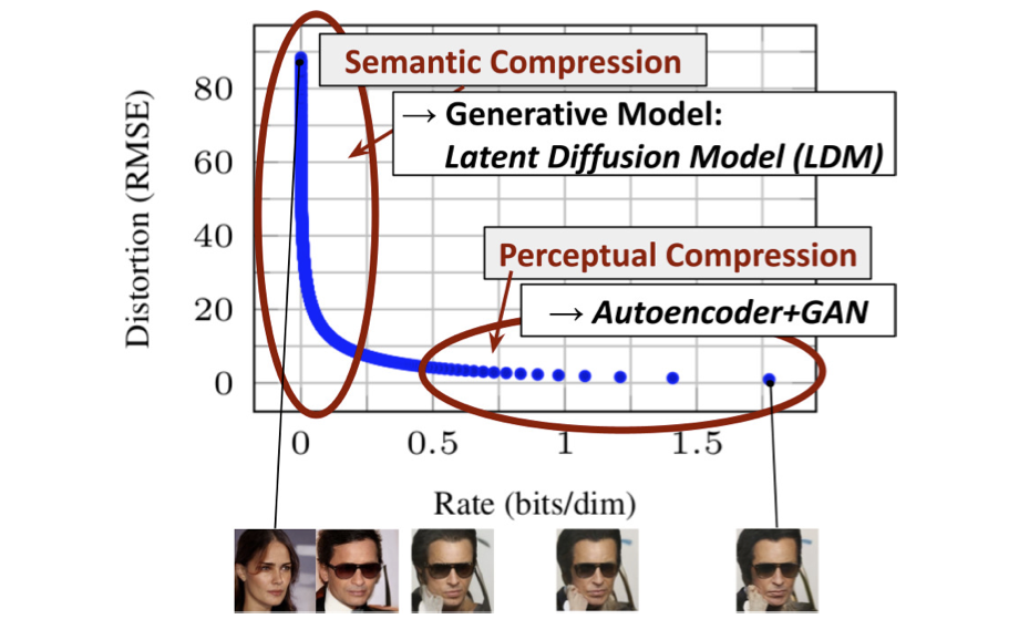
Figure 2. Illustrating perceptual and semantic compression: Most bits of a digital image correspond to imperceptible details. While DMs allow to suppress this semantically meaningless information by minimizing the responsible loss term, gradients (during training) and the neural network backbone (training and inference) still need to be evaluated on all pixels, leading to superfluous computations and unnecessarily expensive optimization and inference. We propose latent diffusion models (LDMs) as an effective generative model and a separate mild compression stage that only eliminates imperceptible details. Data and images from [30].

1. 지각적 압축 단계(Perception Compression)로 빈도가 높은 세부 정보를 제거하지만 의미적 변화는 거의 학습하지 않음
2. 실제 생성 모델이 데이터의 의미적 및 개념적 구성을 학습(Semantic Compression). 지각적으로는 동등하지만 계산적으로는 더 적합한 공간을 찾아 고해상도 이미지 합성을 위한 차이 모델을 훈련

훈련을 두 단계로 분리

1. 데이터 공간과 지각적으로 동등한 저차원(따라서 효율적인) 표현 공간을 제공하는 자동 인코더를 훈련
2. 공간 차원과 관련하여 더 나은 확장 특성을 보이는 학습된 잠재 공간에서 DM을 훈련, 지속적인 공간 압축에 의존할 필요가 없음. 복잡성이 감소하여 단일 네트워크 패스로 잠재 공간에서 효율적인 이미지 생성이 가능. (LDM)

범용 자동 인코딩 단계를 한 번만 훈련 → 여러 DM 훈련에 재사용하거나 완전히 다른 작업을 탐색할 수 있음

트랜스포머를 DM의 UNet 백본에 연결, 유형의 토큰 기반 컨디셔닝 메커니즘을 가능하게 하는 아키텍처를 설계

Method

diffusion model에 training에서 high quality를 위한 computational cost를 낮추기 위해 undersampling 사용 → 하지만, 픽셀 공간에서 이미지를 생성하는 과정은 여전히 많은 계산 자원을 필요

undersampling : 전체 데이터 중에서 일부만 선택하여 사용하는 방법, 주로 데이터의 특정 부분을 무시하거나 덜 중요하게 처리함으로써 처리 속도를 높이고 계산 자원을 절약하는 데 사용

따라서 auto-encoder 사용

---

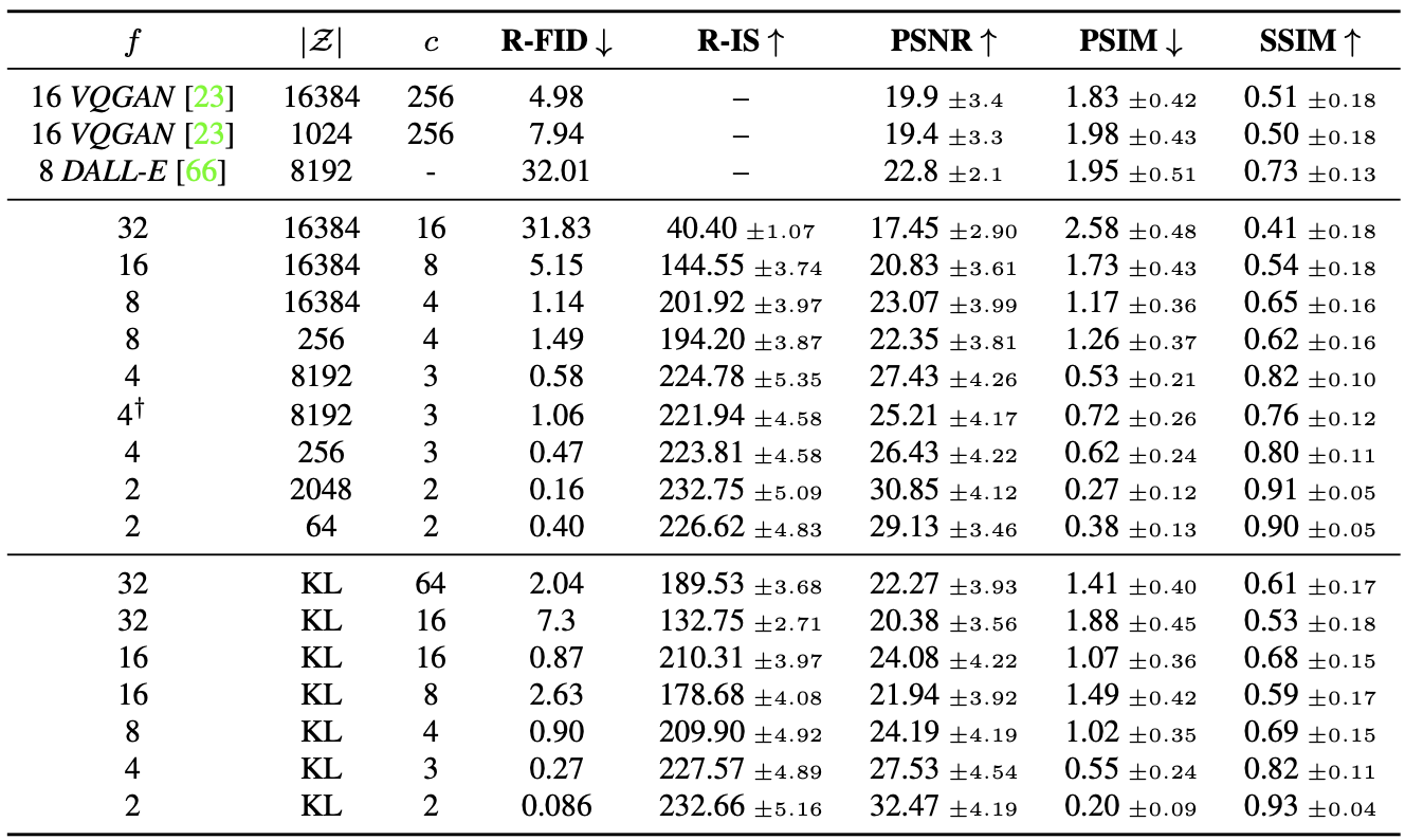
Perceptual Image Compression (AutoEncoder)

Perceptual Loss

\[\mathcal{L}_{\text{perceptual}} = \frac{1}{CHW} \sum_{c=1}^{C} \sum_{h=1}^{H} \sum_{w=1}^{W} \left( \phi(x)_{c,h,w} - \phi(\hat{x})_{c,h,w} \right)^2\]

\(\mathcal{L}_{perceptual}\) : 지각적 손실 함수

\(ϕ(x)$와 $ϕ(\hat{x})\)는 사전 훈련된 신경망에서 추출한 원본 이미지

\(x\) 와 생성된 이미지 \(\hat{x}\) 의 특징 맵

C는 특징 맵의 채널 수, H는 높이, W는 너비

\(ϕ(x)_{c,h,w}\) 와 \(ϕ(\hat{x})_{c,h,w}\) 는 채널 c, 높이 h, 너비 w위치에서의 특징 맵 값

Encoder and Decoder

\(x ∈ R^{H×W×3}\) → \(z = ε(x)\) , \(z ∈ R^{h×w×c}\) → \(x = D(z) = D(ε(x))\)

ε : encoder

D : decoder

\(f = H/h = W/w\) : the encoder downsamples the image by a factor

\(f = 2^m\) , with \(m ∈ \mathbb{N}\) : downsampling factors → 이미지의 해상도를 조정하는 중요한 결정 요소

• 다른 sampling factor를 사용하는 이유
  1. 동일한 샘플링 팩터를 사용하는 경우, 모델은 특정 해상도에서만 최적화.
  2. 다양한 샘플링 팩터를 사용하면 모델이 다양한 해상도에서 학습할 수 있게 되어, 실제 상황에서 다양한 조건의 데이터를 처리하는 데 유리
  3. VAE와 같은 모델에서 잠재 공간(latent space)의 크기와 구조는 데이터의 복잡성과 다양성을 반영. 샘플링 팩터가 동일하면 잠재 공간의 표현이 제한.

  다양한 샘플링 팩터를 사용 → 잠재 공간이 더 풍부하고 유의미한 표현을 가짐, 복잡한 데이터 구조를 더 잘 학습

latent space의 고분산을 방지하기 위해 사용된 두 가지 정규화 기법

1. KL 정규화(KL-reg.) : Variational Autoencoder (VAE)에서 사용되는 방법과 유사

   학습된 잠재 공간을 표준 정규 분포에 가까워지도록 하는 KL-패널티(Kullback-Leibler Divergence)를 부과

2. 벡터 양자화 정규화(VQ-reg.) : 벡터 양자화(Vector Quantization) 레이어를 디코더에 포함시켜 사용

   VQGAN(Vector Quantized Generative Adversarial Network)과 유사하지만, 양자화 레이어가 디코더에 흡수되어 있다는 차이

   양자화 레이어는 학습된 잠재 공간을 제한된 수의 고정된 벡터로 표현하여 고분산을 억제

여기서는 VQGAN을 사용

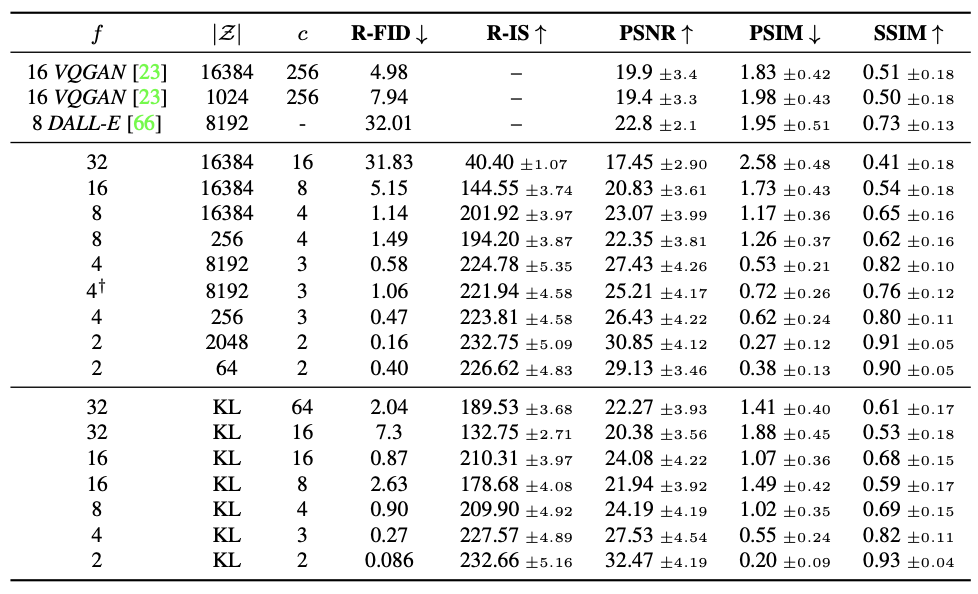
이 모델은 학습된 잠재 공간 $z=E(x)$ 의 2차원 구조를 활용하여 상대적으로 낮은 압축률을 사용하면서도 매우 우수한 복원 성능을 달성 → 이전 연구들은 학습된 잠재 공간을 임의의 1차원 순서로 배열하여 분포를 모델링했기 때문에, 잠재 공간의 내재된 구조를 무시

→ 원본 이미지의 중요한 특징을 더 잘 복원 (아마 이미지이기 때문에 2차원?)

---

Latent Diffusion Models

• Diffusion Models (DDPM)

  \[L_{DM} = \mathbb{E}_{x, \epsilon \sim \mathcal{N}(0,1), t} \left[ \left\| \epsilon - \epsilon_\theta (x_t, t) \right\|_2^2 \right]\]

  with t uniformly sampled from {1, . . . , T}

• Generative Modeling of Latent Representations

  \[L_{LDM} := \mathbb{E}_{\mathcal{E}(x), \epsilon \sim \mathcal{N}(0,1), t} \left[ \left\| \epsilon - \epsilon_\theta (z_t, t) \right\|_2^2 \right].\]

  \(ε_θ(◦, t)\) 은 UNet으로 구현

---

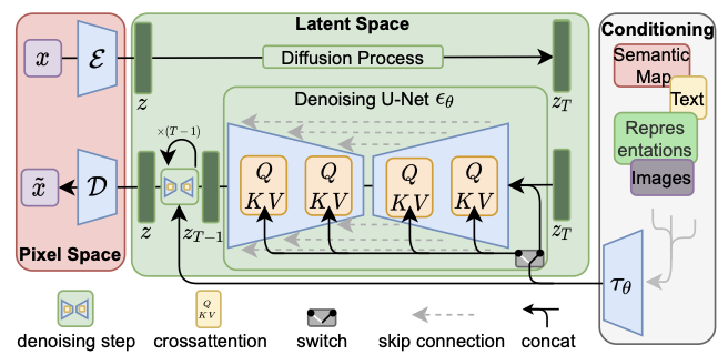
Conditioning Mechanisms

원칙적으로 $p(z

y)$ 형식의 조건부 분포를 모델링 → 조건부 노이즈 제거 자동 인코더 $ε_θ(z_t, t, y)$로 구현

다양한 입력 모달리티의 Attention based 모델을 학습하는 데 효과적인 교차 주의 메커니즘으로 기본 UNet 백본을 보강하여 Diffusion Model을 보다 유연한 conditional image generator로 전환

domain specific encoder \(τ_θ$ : $τ_θ(y) ∈ R^{M×d_τ}\)

UNet에 cross-attention

\[\text{Attention}(Q, K, V) = \text{softmax}\left(\frac{QK^T}{\sqrt{d}}\right) \cdot V\] \[Q = W_Q^{(i)} \cdot \varphi_i(z_t), \quad K = W_K^{(i)} \cdot \tau_\theta(y), \quad V = W_V^{(i)} \cdot \tau_\theta(y). \\\]

\(\varphi_i(z_t) \in \mathbb{R}^{N \times d_{\epsilon}^i}\) : φi는 i번째 층 또는 모듈(UNet)에서 생성된 중간 특징 벡터

\(\epsilon_\theta \text{ and } W_V^{(i)} \in \mathbb{R}^{d \times d_\epsilon^i}, \quad W_Q^{(i)} \in \mathbb{R}^{d \times d_\tau} \quad \& \quad W_K^{(i)} \in \mathbb{R}^{d \times d_\tau} \quad\): learnable projection matrices

\(\epsilon_\theta\) : 모델에서 예측한 잡음(noise)을 나타내는 변수, θ는 모델의 매개변수

• Query : 현재의 입력이 다른 입력과 얼마나 관련이 있는지 측정하는 데 사용 , \(\varphi_i(z_t)\) 을 사용
• Key : Query와의 관련성을 평가하는 기준 , \(τ_θ\) 을 사용
• Value : 최종 출력에 포함될 정보 , \(τ_θ\) 을 사용

cross attention을 통해 domain specific encoder의 출력을 내보냄

최종 수식

\[L_{LDM} := \mathbb{E}_{\mathcal{E}(x), y, \epsilon \sim \mathcal{N}(0,1), t} \left[ \left\| \epsilon - \epsilon_\theta (z_t, t, \tau_\theta (y)) \right\|_2^2 \right]\]

Experiments

On Perceptual Compression Tradeoffs

different downsampling factors f ∈ {1, 2, 4, 8, 16, 32}을 확인

LDM-f (latent space) , LDM-1 (pixel space)

Figure 6. Analyzing the training of class-conditional LDMs with different downsampling factors f over 2M train steps on the Im- ageNet dataset. Pixel-based LDM-1 requires substantially larger train times compared to models with larger downsampling factors (LDM-{4-16}). Too much perceptual compression as in LDM-32 limits the overall sample quality. All models are trained on a single NVIDIA A100 with the same computational budget. Results obtained with 100 DDIM steps [84] and κ = 0.

LDM-{1,2}의 다운샘플링 인자가 작으면 훈련 진행 속도가 느려지는 반면, ii) f 값이 지나치게 크면 비교적 적은 훈련 단계 후에 충실도가 저하되는 것을 알 수 있습니다

위의 분석(그림 1과 2)을 다시 살펴보면, 이는 i) Semantic Compression의 대부분을 확산 모델에 맡기고, ii) 너무 강한 첫 단계 압축으로 인해 정보가 손실되어 품질 저하 발생

LDM-{4-16}은 효율성과 지각적으로 충실한 결과 사이의 균형을 잘 맞추고 있으며, 이는 2M 훈련 단계 이후 픽셀 기반 확산(LDM-1)과 LDM-8 사이의 유의미한 FID 격차 38로 나타납니다.

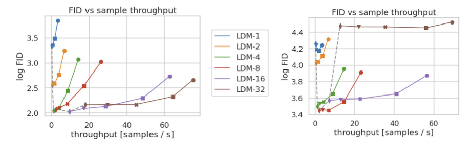
Figure 7. Comparing LDMs CelebA-HQ (left) and ImageNet (right) datasets. Different markers indicate {10, 20, 50, 100, 200} sampling steps using DDIM, from right to left along each line. The dashed line shows the FID scores for 200 steps, indicating the strong performance of LDM- {4-8}. FID scores assessed on 5000 samples. All models were trained for 500k (CelebA) / 2M (ImageNet) steps on an A100.

픽셀 기반에 비해 확실히 빠른 처리속도

이미지넷과 같은 복잡한 데이터 세트는 품질 저하를 피하기 위해 압축률을 낮추는게 좋음

LDM-4와 -8이 베스트

Image Generation with Latent Diffusion

Uncondition result

Table 1. Evaluation metrics for unconditional image synthesis. CelebA-HQ results reproduced from [43, 63, 100], FFHQ from [42, 43]. † : N -s refers to N sampling steps with the DDIM [84] sampler. ∗: trained in KL-regularized latent space. Additional results can be found in the supplementary.

text condition

Table 2. Evaluation of text-conditional image synthesis on the 256 × 256-sized MS-COCO [51] dataset: with 250 DDIM [84] steps our model is on par with the most recent diffusion [59] and autoregressive [26] methods despite using significantly less pa- rameters. †/∗:Numbers from [109]/ [26]

latent space에서는 매개 변수의 절반을 사용하고 4배 적은 훈련 리소스를 다시 사용함 그럼에도 성능이 더 좋음

Figure 4. Samples from LDMs trained on CelebAHQ [39], FFHQ [41], LSUN-Churches [102], LSUN-Bedrooms [102] and class-conditional ImageNet [12], each with a resolution of 256 × 256. Best viewed when zoomed in. For more samples cf . the supplement.

Conditional Latent Diffusion

Transformer Encoders for LDMs

LDM에 cross attention을 도입해 다양한 condition을 받을 수 있도록 함

BERT-토큰라이저를 사용하고 τθ를 변환기로 구현하여 (multi head) cross attention를 통해 UNet에 매핑되는 잠재 코드를 추론

언어 표현 학습을 위한 BERT-토큰라이저와 시각적 합성을 위한 diffusion의 조합

classifier-free diffusion guidance를 적용하면 샘플의 품질이 크게 향상 (LDM-KL-8-G) 동시에 파라미터 수를 크게 줄임

Convolutional Sampling Beyond $256^2$

공간적으로 정렬된 컨디셔닝 정보를 εθ의 입력에 연결 → LDM은 효율적인 범용 이미지 간 번역 모델로 사용

의미론적 합성 : 풍경 이미지와 의미론적 지도(semantic maps)를 사용

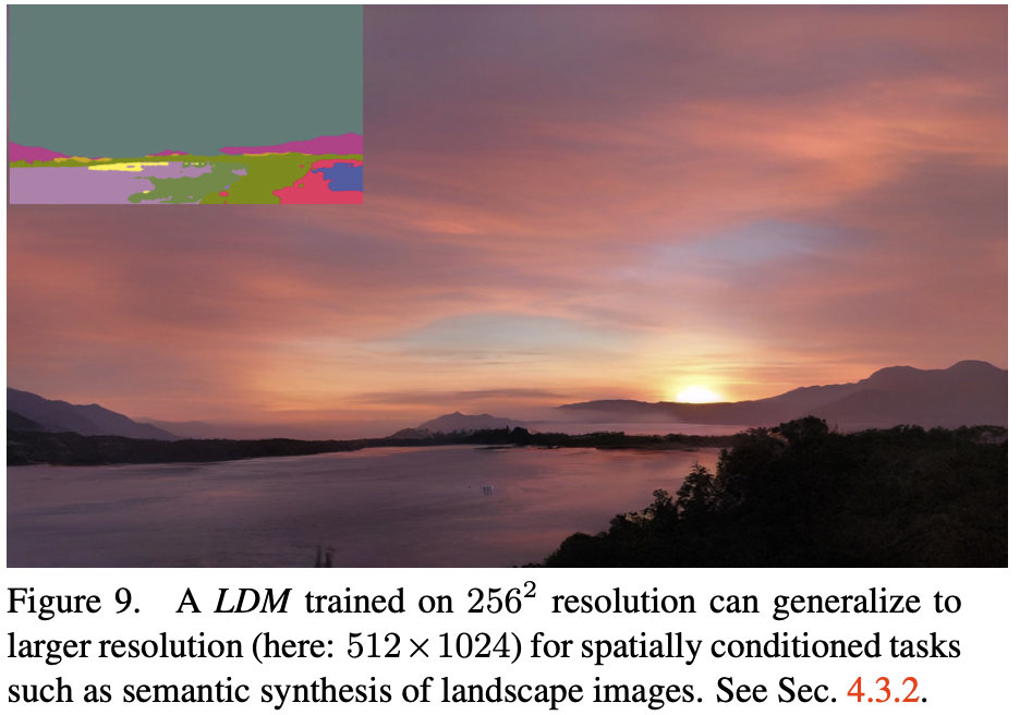
256x256 해상도에서 훈련하지만, 모델은 더 큰 해상도에서도 일반화될 수 있으며, 메가픽셀 크기의 이미지도 생성 가능

Super-Resolution with Latent Diffusion

Figure 10. ImageNet 64→256 super-resolution on ImageNet-Val. LDM-SR has advantages at rendering realistic textures but SR3 can synthesize more coherent fine structures. See appendix for additional samples and cropouts. SR3 results from [72].

‘concatenation’을 통해 저해상도 이미지에 직접 컨디셔닝함으로써 LDM을 효율적으로 초해상도로 훈련

일부러 저해상도로 낮춰서 resolution을 진행

• 실험:
  • SR3[72] 모델을 따라 4배 다운샘플링을 통해 이미지를 low-resolution시키고, 이를 interpolation으로 수정합니다.
  • SR3의 데이터 처리 파이프라인을 따르며, ImageNet 데이터셋에서 모델을 훈련합니다.
  • OpenImages에서 사전 학습된 f = 4 오토인코딩 모델(VQ-regularization, 표 8 참조)을 사용하고, 저해상도 컨디셔닝 정보(y)와 UNet의 입력을 연결합니다.
• 결과:
  • 정성적(qualitative) 및 정량적(quantitative) 결과 경쟁력 있는 성능을 확인
  • LDM-SR 모델은 FID(Frechet Inception Distance) 점수에서 SR3보다 우수하지만, SR3는 IS(Inception Score)에서 더 우수
  • 단순 이미지 회귀 모델은 가장 높은 PSNR(피크 신호 대 잡음비) 및 SSIM(구조적 유사성 지수) 점수를 달성하지만, 이러한 지표는 사람의 인식과 잘 맞지 않으며, 고주파 디테일이 불완전하게 정렬된 것보다 흐릿함을 선호하는 경향이 있습니다[72].

Table 5. ×4 upscaling results on ImageNet-Val. (2562); †: FID features computed on validation split, ‡: FID features computed on train split; ∗: Assessed on a NVIDIA A100

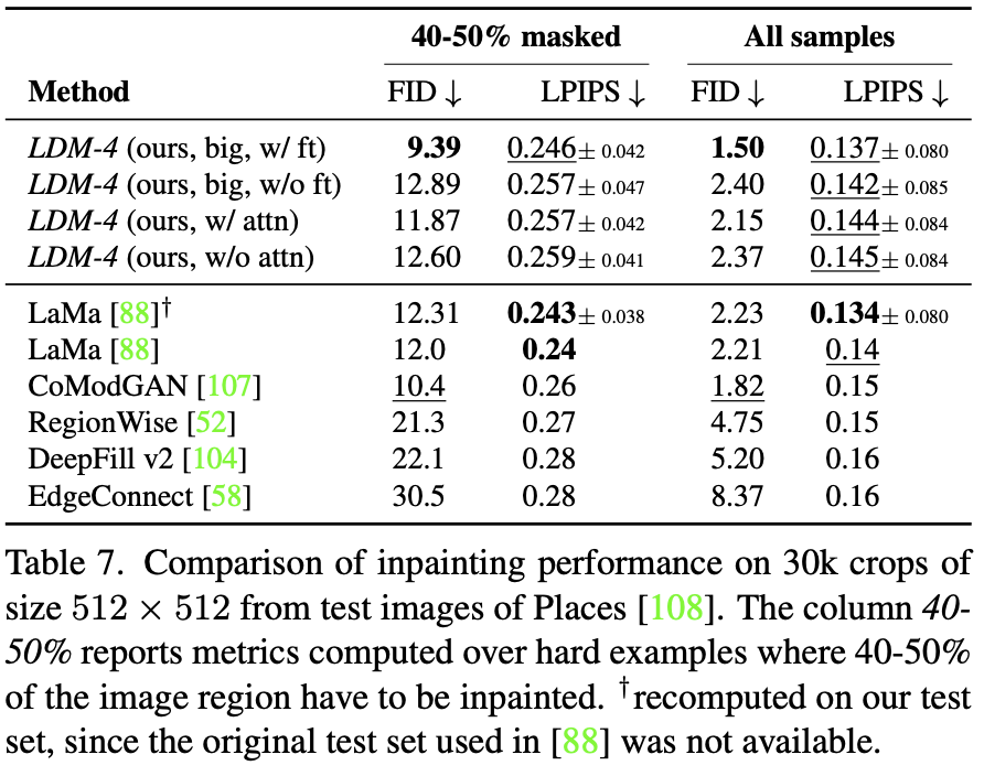
Table6. Assessing inpainting efficiency.†:Deviations from Fig.7 due to varying GPU settings/batch sizes cf . the supplement.

D.6. Super-Resolution : Appendix 에 추가로 있음

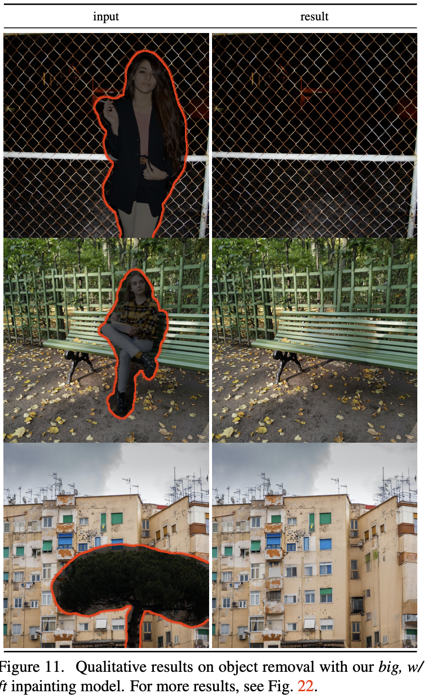
Inpainting with Latent Diffusion

E.2.2 Inpainting : Appendix 에 추가로 있음

Limitations & Societal Impact

순차 샘플링 프로세스는 여전히 GAN보다 느림

높은 정밀도가 요구되는 경우 LDM의 사용에 의문

Appendix

D.4. Class-Conditional Image Synthesis on ImageNet

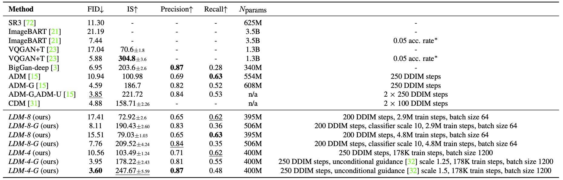
Table10. Comparison of a class-conditional ImageNet LDM with recent state-of-the-art methods for class-conditional image generation on the ImageNet [12] dataset.∗: Classifier rejection sampling with the given rejection rate as proposed in [67].

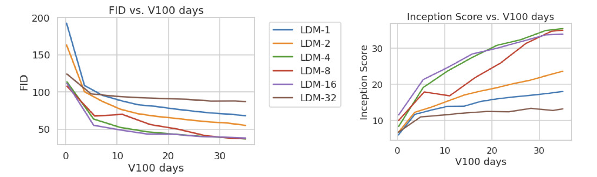
D.5. Sample Quality vs. V100 Days (Continued from Sec. 4.1)

E. Implementation Details and Hyperparameters

Hyperparameters

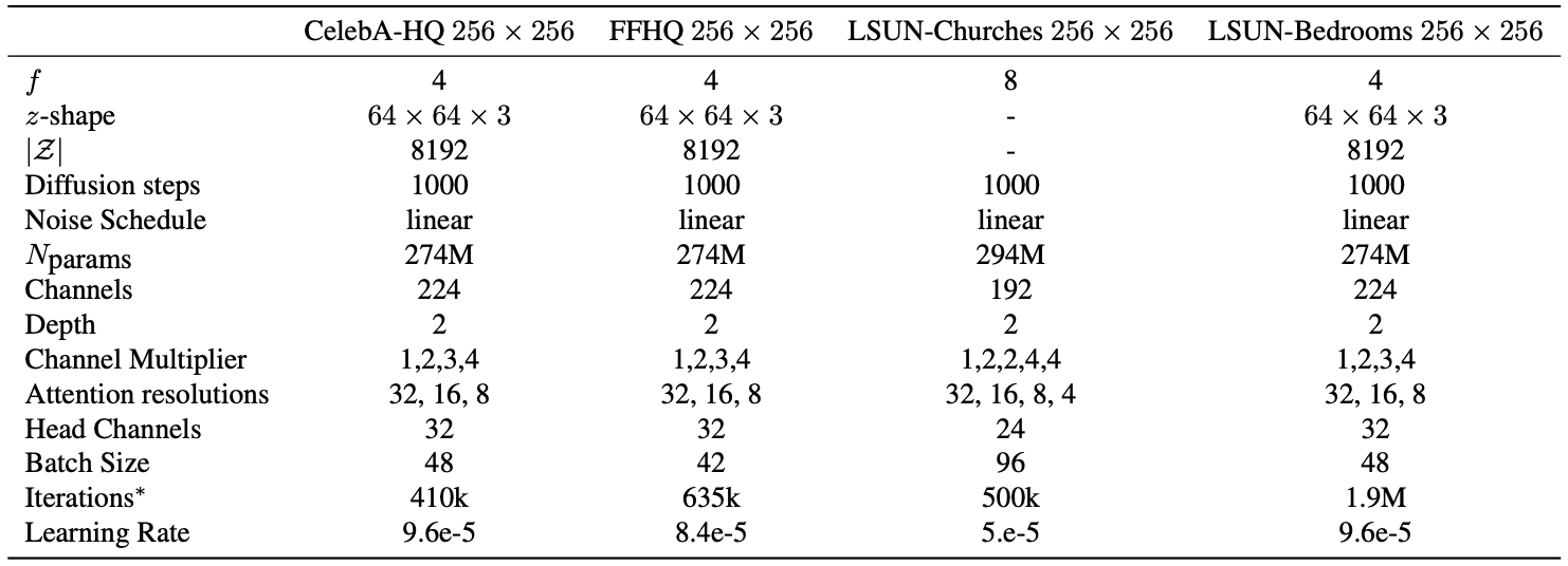
Table12. Hyper parameters for the unconditional LDMs producing the numbers shown in Tab.1. All models trained on a single NVIDIA A100.

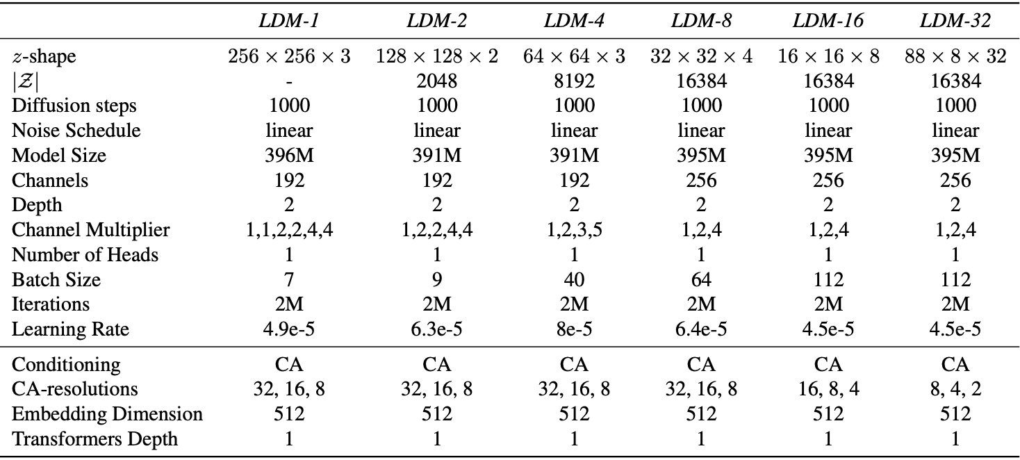
Table13. Hyper parameters for the conditional LDMs trained on the ImageNet dataset for the analysis in Sec.4.1. All models trained on a single NVIDIA A100.

E.2. Implementation Details

Implementations of $τ_θ$ for conditional LDMs

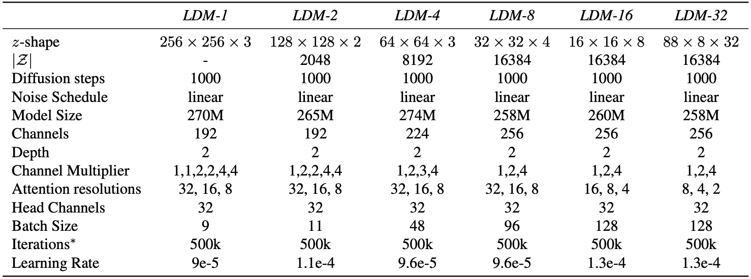
Table14. Hyperparameters for the unconditional LDMs trained on the CelebA dataset for the analysis in Fig.7. All models trained on a single NVIDIA A100. ∗: All models are trained for 500k iterations. If converging earlier, we used the best checkpoint for assessing the provided FID scores.

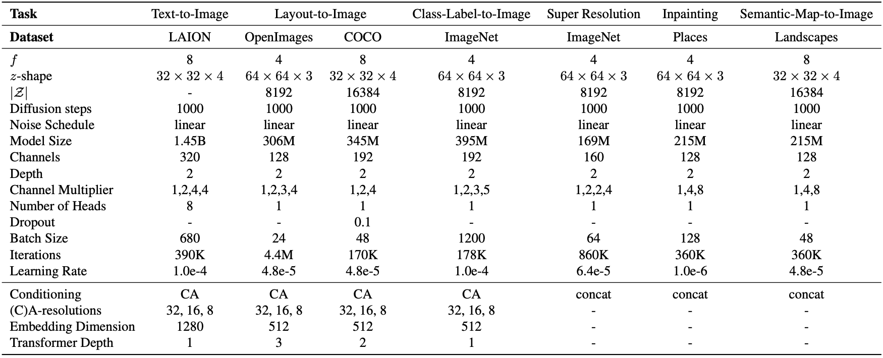
Table15. Hyperparameters for the conditional LDMs from Sec.4. All models trained on a single NVIDIA A100 except for the in painting model which was trained on eight V100.

\[\zeta \leftarrow \text{TokEmb}(y) + \text{PosEmb}(y) \ \ \ \ \ \ \text{for } i = 1, \ldots, N \text{ :} \\\quad \zeta_1 \leftarrow \text{LayerNorm}(\zeta) \\\quad \zeta_2 \leftarrow \text{MultiHeadSelfAttention}(\zeta_1) + \zeta \\\quad \zeta_3 \leftarrow \text{LayerNorm}(\zeta_2) \\\quad \zeta \leftarrow \text{MLP}(\zeta_3) + \zeta_2 \\\zeta \leftarrow \text{LayerNorm}(\zeta)\]

Table16. Architecture of a transformer block as described in Sec.E.2.1, replacing the self-attention layer of the standard “ablated UNet” architecture [15]. Here, $n_h$ denotes the number of attention heads and d the dimensionality per head.

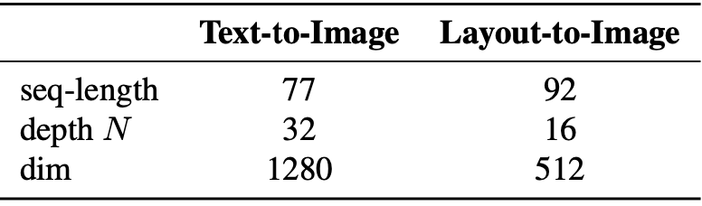
Table17. Hyperparameters for the experiments with transformer encoders in Sec.4.3.