[논문분석] Real Time Speech Enhancement in the Waveform Domain
Abstract
We present a causal speech enhancement model working on the raw waveform that runs in real-time on a laptop CPU. The proposed model is based on an encoder-decoder architecture with skip-connections. It is optimized on both time and frequency domains, using multiple loss functions. Empirical evidence shows that it is capable of removing various kinds of background noise including stationary and non-stationary noises, as well as room reverb. Additionally, we suggest a set of data augmentation techniques applied directly on the raw waveform which further improve model performance and its generalization abilities. We perform evaluations on several standard benchmarks, both using objective metrics and human judgements. The proposed model matches state-of-the-art performance of both causal and non causal methods while working directly on the raw waveform. Index Terms: Speech enhancement, speech denoising, neural networks, raw waveform
1. Introduction
DEMUCS라는 기존 딥러닝 모델을 실시간 음성 향상에 맞게 새롭게 변형한 모델을 제안
- 실시간 처리: 딜레이를 최소화한 인과적(causal) 모델로 설계
- 고효율: 일반 노트북 CPU 코어 하나에서도 실시간보다 빠르게 작동
- 고품질: U-Net과 유사한 구조를 사용하여 소음이 섞인 음성 파형(waveform)을 직접 입력받아 깨끗한 파형을 출력
- 고급 학습 기법: 두 가지 종류의 손실 함수(L1 손실, 스펙트로그램 손실)와 데이터 증강(주파수 대역 마스킹, 잔향 추가)을 통해 모델의 성능을 극대화
2. Model
2.1. Notations and problem settings
monaural (single-microphone) speech enhancement 과제 해결
- 입력 신호
x는 깨끗한 음성y에 배경 소음n이 더해진 상태(x = y + n)라고 가정 - 목표는 소음이 섞인
x를 입력받아 깨끗한 음성y와 거의 동일한 결과물을 출력하는 함수(모델)f를 만드는 것 → f(x) ≈ y 최종 목표 - music source separation에 사용했던 DEMUCS 구조를 가져와서 사용
2.2. DEMUCS architecture
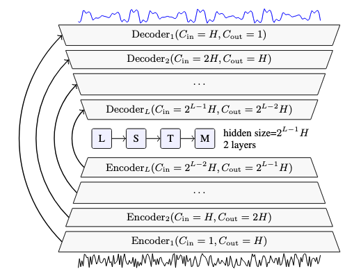
(a) Causal DEMUCS with the noisy speech as input on the bottom and the clean speech as output on the top. Arrows represents UNet skip connections. H controls the number of channels in the model and L its depth.
(b) View of each encoder (bottom) and decoder layer (top). Arrows are connections to other parts of the model. Cin (resp. Cout) is the number of input channels (resp. output), K the kernel size and S the stride.
Figure 1: Causal DEMUCS architecture on the left, with detailed representation of the encoder and decoder layers on the right. The on the fly resampling of the input/output by a factor of U is not represented.
DEMUCS는 인코더-디코더 구조에 U-Net의 스킵 커넥션(skip connection)을 결합
- 인코더 (Encoder)
- 소음이 섞인 원본 음성 파형(waveform)을 입력으로 사용
- Multi-layer convolution 층을 거치면서 음성 신호를 점차 압축하여 핵심적인 특징(latent representation)을 추출
- 중간 네트워크 (Sequence Modeling)
- 인코더가 압축한 특징을 LSTM 네트워크에 통과시켜 시간의 흐름에 따른 음성의 패턴을 학습합니다.
- 핵심: 실시간 처리가 가능하도록 단방향(unidirectional) LSTM을 사용합니다. (실시간이 아닌 경우엔 양방향 LSTM 사용)
- 디코더 (Decoder)
- LSTM이 처리한 특징을 다시 여러 개의 전치 컨볼루션(transposed convolution) 층을 통해 음성 파형을 복원
- Skip Connection
- 기존 정보 보존
- 학습 단순화 - 차이만을 학습
2.3. Objective
두 가지 종류의 손실 함수를 조합하여 사용
Overall Loss Function
\[\mathcal{L}_{\text{total}} = \frac{1}{T} \left[ \|y - \hat{y}\|_1 + \sum_{i=1}^{M} \mathcal{L}_{\text{stft}}^{(i)}(y, \hat{y}) \right]\]$\|y - \hat{y}\|_1$(파형 손실): L1 손실을 의미합니다.- y: 원본의 깨끗한 음성 신호 (정답)
- haty: 모델이 출력한 음성 신호 (예측)
- 의미: 두 음성 파형을 샘플 하나하나 직접 비교하여 그 차이의 절댓값 합을 줄임 즉, 모델의 출력 파형이 정답 파형과 모양 자체가 최대한 비슷해지도록 유도
$\sum_{i=1}^{M} \mathcal{L}_{\text{stft}}^{(i)}(y, \hat{y})$(다중 해상도 STFT 손실)- $\mathcal{L}_\text{stft}$: 주파수 영역에서 신호를 비교하는 STFT 손실입니다.
- $\sum_{i=1}^{M}$: 하나의 기준이 아닌, M개의 서로 다른 설정으로 STFT 손실을 여러 번 계산하여 모두 더한다는 의미 이를 통해 다양한 관점에서 주파수 특성을 비교하여 음질을 높임
STFT loss components
\[\mathcal{L}_{\text{stft}}(y, \hat{y}) = \mathcal{L}_{\text{sc}}(y, \hat{y}) + \mathcal{L}_{\text{mag}}(y, \hat{y})\]-
스펙트럼 수렴 손실 (Spectral Convergence Loss, $\mathcal{L}_\text{sc}$)
\[\mathcal{L}_{\text{sc}}(y, \hat{y}) = \frac{\big\| |STFT(y)| - |STFT(\hat{y})| \big\|_F}{\| |STFT(y)| \|_F}\]$|STFT(y)|$: 신호 y를 STFT(단시간 푸리에 변환)하여 얻은 스펙트로그램의 크기(magnitude)$∣\cdot∣_F$: 프로베니우스 노름(Frobenius Norm)으로, 행렬의 모든 원소를 제곱하여 더한 후 제곱근을 취한 값- 정답 스펙트로그램과 예측 스펙트로그램의 크기가 전반적으로 얼마나 다른지를 정규화하여 측정 → 주파수 에너지 분포가 비슷해지도록
-
크기 손실 (Magnitude Loss, $\mathcal{L}_\text{mag}$)
\[\mathcal{L}_{\text{mag}}(y, \hat{y}) = \frac{1}{T} \big\| \log|STFT(y)| - \log|STFT(\hat{y})| \big\|_1\]$\log|STFT(y)|$: 스펙트로그램 크기에 로그(log)를 적용 → 사람의 청각 특성에 더 가까운 비교$∣\cdot∣_1$: L1 노름으로, 각 원소 간 차이의 절댓값을 모두 더한 값- 사람이 인지하는 주파수별 소리 크기의 차이를 줄이는 데 집중 → 사람이 듣기에 더 자연스러운 소리
3. Experiments
3.1. Implementation details
Evaluation Methods
객관적 평가지표
- PESQ: 사람이 인지하는 음질을 예측하는 점수 (0.5 ~ 4.5점).
- STOI: 음성의 명료도(얼마나 잘 들리는지)를 나타내는 점수 (0 ~ 100점).
- CSIG, CBAK, COVL: 사람이 평가할 평균 점수(MOS)를 예측하는 모델입니다.
- CSIG: 음성 자체의 왜곡 수준 예측.
- CBAK: 배경 소음이 얼마나 거슬리는지 예측.
- COVL: 전반적인 품질 예측.
주관적 평가지표
MOS (평균 의견 점수): 실제 사람들이 직접 듣고 음질에 1~5점 척도로 점수를 매기는 방식
Training
- 데이터셋: Valentini 데이터셋은 400 에포크(epoch), DNS 데이터셋은 250 에포크 동안 학습
- 손실 함수: 기본적으로 L1 손실을 사용했고, Valentini 데이터셋에서는 추가로 STFT 손실을 0.5의 가중치 계산
- 옵티마이저: Adam 옵티마이저를 특정 파라미터(학습률 3e-4 등)로 설정
- 샘플링 레이트: 모든 오디오는 16kHz로 처리
Model
- 비-실시간(Non-causal) DEMUCS: 성능 비교를 위한 기준 모델.
- U =2, S=2, K=8, L=5, H=64
- 실시간(Causal) DEMUCS (H=48): 효율성을 높인 가벼운 실시간 모델.
- U =4, S=4, K=8, L=5, H=48
- 실시간(Causal) DEMUCS (H=64): 성능을 높인 무거운 실시간 모델.
- U =4, S=4, K=8, L=5, H=64
Data Normalization
standard deviation으로 정규화
오디오 전체가 아닌 현재까지 들어온 데이터만으로 표준편차를 계속 추정
causal DEMUCS 모델은 37ms 크기의 오디오 프레임을 16ms 간격으로 처리
Data augmentation
- Random Shift: 오디오를 시간 축에서 무작위로 미세하게 이동
- Remix: 한 배치 내의 음성과 소음을 서로 섞음
- BandMask: 주파수 영역에서 특정 대역을 무작위로 제거하여 모델이 일부 정보가 없을 때도 잘 작동하도록 훈련
- batch 내에서 멜 스케일(mel scale)을 기준, 주파수 영역의 20%를 무작위로 선택하여 제거
- Revecho: 인공적인 울림(reverb)과 메아리(echo)를 추가
λ(람다), 초기 이득:[0, 0.3]범위에서 무작위로 선택 → 메아리의 크기가 원본 소리의 0% ~ 30% 사이에서 결정된다는 의미τ(타우), 초기 딜레이:[10, 30] ms범위에서 무작위로 선택 → 메아리 기본 시간 간격RT60, 잔향 시간:[0.3, 1.3]초 범위에서 무작위로 선택 → 소리가 60데시벨만큼 감쇠하는 데 걸리는 시간, 공간의 울림 정도 0.3초는 작은 방, 1.3초는 비교적 큰 홀의 울림을 시뮬레이션N: 생성되는 총 메아리의 개수ρ: 감쇠 계수$ρ^N ≤ 1e-3$: 메아리 생성을 멈추는 종료 조건,N번째 메아리의 크기가 원본의 0.1% 이하로 작아져 거의 들리지 않게 되면 메아리 생성을 중단
- 모든 데이터셋: Random Shift는 기본적으로 적용
- Valentini 데이터셋: Remix와 BandMask를 사용
- DNS 데이터셋: 울림(reverb) 환경이 중요한 벤치마크이므로 Revecho 기법만 사용
Causal streaming evaluation
실제 스트리밍 환경에 적용할 구체적인 방법들
Cumulative Standard Deviation
- 스트림의 시작부터 현재 시점까지 들어온 데이터만으로 표준편차를 계속해서 다시 계산
Lookahead and Buffering
- 아주 잠깐(3ms) 미래의 오디오를 미리 볼 수 있도록 허용 → 성능 향상
- 이로 인해 총 처리 프레임 크기는 40ms
Padding Trick using ‘Invalid’ Output
- 오디오 처리시, 맨 끝부분의 출력은 부정확하고 ‘무효(invalid)’한 값
- 이를 버리지 않고, 다운샘플링 과정의 패딩(padding)으로 재활용
- 음질 점수 향상
Efficient Implementation
- 처리하는 오디오 프레임들은 서로 겹치는 부분을 Caching 하여 중복 제거
- PyTorch만을 사용
3.2. Results
SOTA 모델인 DeepMMSE와 유사한 성능
![Table 1: Objective and Subjective measures of the proposed method against SOTA models using the Valentini benchmark [18].](/assets/Images/2025-07-20-DEMUCS/image%202.png)
Table 1: Objective and Subjective measures of the proposed method against SOTA models using the Valentini benchmark [18].
Dry/Wet 조절 기능: (dry * 원본 잡음) + ((1-dry) * 잡음 제거된 음성) 처럼 약간의 원본 소리를 섞어주니(예: 5%), 인공적인 느낌이 줄어들어 오히려 사람이 인지하는 전반적인 품질이 향상
![Table 2: Subjective measures of the proposed method with different treatment of reverb, on the DNS blind test set [19]. Recordings are divided in 3 categories: no reverb, reverb (artificial) and real recordings. We report the OVL MOS. All models are causal. For DEMUCS , we take U =4, H=64 and S=4.](/assets/Images/2025-07-20-DEMUCS/image%203.png)
Table 2: Subjective measures of the proposed method with different treatment of reverb, on the DNS blind test set [19]. Recordings are divided in 3 categories: no reverb, reverb (artificial) and real recordings. We report the OVL MOS. All models are causal. For DEMUCS , we take U =4, H=64 and S=4.
DNS 데이터셋 결과: 인공적인 울림(reverb)이 포함된 데이터에서는, 울림을 완전히 제거하는 것보다 부분적으로 제거하는 것이 더 좋은 평가를 받음 → 완전히 제거하면 왜곡 발생
3.3. Ablation
![Table 3: Ablation study for the causal DEMUCS model with H=64, S=4, U =4 using the Valentini benchmark [18].](/assets/Images/2025-07-20-DEMUCS/image%204.png)
Table 3: Ablation study for the causal DEMUCS model with H=64, S=4, U =4 using the Valentini benchmark [18].
3.4. Real-Time Evaluation
Real-Time Factor, RTF
RTF < 1: 실시간보다 빠름 (목표)RTF > 1: 실시간보다 느림 (딜레이 발생)
쿼드코어 Intel i5 CPU에서 테스트 진행
- 무거운 모델 (H=64 버전): RTF = 1.05
- 가벼운 모델 (H=48 버전): RTF = 0.6
- 가벼운 모델 (단일 코어 환경): RTF = 0.8
3.5. The effect on ASR models
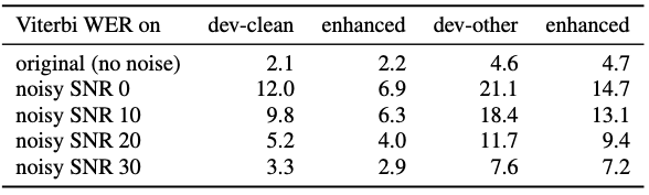
Table 4: ASR results with a state-of-the-art acoustic model, Word Error Rates without decoding, no language model. Results on the LIBRISPEECH validation sets with added noise from the test set of DNS, and enhanced by DEMUCS .
소음 제거 기술이 ASR 성능을 크게 향상시킴
가장 시끄러운 환경(SNR 0)에서는 소음으로 인해 발생한 에러의 51%를 복구했으며, 평균적으로 30~40%의 에러를 복구
후속 연구
1. Hybrid Demucs
https://arxiv.org/abs/2111.03600
https://arxiv.org/pdf/2211.08553
- DEMUCS의 문제점: 오직 파형(Waveform) 영역에서만 동작
- 이 방식은 음질은 좋지만, 복잡하게 얽힌 소리나 특정 주파수 대역에 집중된 노이즈를 정밀하게 분리하는 데 한계 → 미세한 왜곡이나 인공적인 소음(artifact)이 남음
- 개선 방식: 주파수(Spectrogram) 영역을 처리하는 분기를 추가하여 두 방식을 결합(Hybrid)
- 파형 영역에서는 전체적인 음질과 시간적 연속성을 잡고,
- 주파수 영역에서는 더 정밀하게 노이즈의 특성을 분석하여 제거
2. FullSubNet 계열
https://arxiv.org/pdf/2010.15508
- DEMUCS의 문제점: 단일 스트림으로 전체 주파수 대역을 한 번에 처리하기 때문에, 광범위한 배경 소음과 특정 주파수에 집중된 돌발 소음이 섞인 복잡한 노이즈 환경에 대한 대처 능력이 상대적으로 부족
- 개선 방식: 오디오 신호를 Full-Band과 Sub-Bands으로 나누어 동시에 처리합니다.
3. 신경망 보코더 기반 모델
https://arxiv.org/pdf/2104.03538
- DEMUCS의 문제점: 근본적으로 ‘소음을 빼는(subtractive)’ 방식이기 때문에, 소음을 제거한 자리에 미세한 왜곡이나 부자연스러움이 남 → 음질의 상한선이 명확
- 개선 방식: 소음을 빼는 대신, 깨끗한 음성을 아예 새로 만들어냅니다(Re-synthesis).
- 소음 섞인 음성에서 깨끗한 음성의 핵심 특징(예: 멜 스펙트로그램)만 추출
- 이 특징을 신경망 보코더(Neural Vocoder)에 넣어 깨끗한 음성 파형을 생성