[프로젝트] AI Spark 글로벌 산불감지 챌린지, TransUNet, Attention U-Net

Inha univ. | 연구개발특구
[Code] , [ProjectPage]

제6회 2024 연구개발특구 AI SPARK 챌린지

Review

이번 인공지능 대회는 처음 참가했으며, 짧은 기간 동안 성능을 높이기 위해 많은 노력을 기울였습니다. 단순히 모델 선정과 구현만 중요한 것이 아니라, 데이터셋을 세밀하게 분석하고, 정확도를 높이기 위한 데이터 전처리 과정의 필요성을 깊이 깨달았습니다. 다음 대회에서는 이를 더욱 철저히 준비할 계획입니다.

높은 성능을 달성하기 위해 기존 모델을 앙상블하는 방법이 좋은 결과를 낸다는 점도 배웠습니다. 단일 모델로 90% 근방의 성능을 달성했지만, 그 이상으로 끌어올리는 데는 어려움을 겪었습니다. 다음 대회에서는 이 부분을 개선하고자 합니다.

또한, 코드 수정 과정에서 과거 버전으로 돌아가야 하는 상황에서 로그 관리의 중요성을 절실히 느꼈습니다. 기존 코드를 덮어쓰는 방식으로 작업하다 보니 어려움이 있었고, 이를 해결하기 위해 버전 관리의 필요성을 깨닫게 되었습니다. Git에 대해 이후 공부했습니다.

약 3주 간에 기록 (24/3/8 ~ 24/3/25)

이전 대회 다른 블로그

제4회 2023 연구개발특구 AI SPARK 챌린지 - 공기압축기 이상 판단

[공모전] 2023 연구개발특구 AI SPARK 챌린지 - 공기압축기 이상 판단

산업용 공기압축기의 이상 유무를 비지도학습 방식을 이용하여 판정
제3회 연구개발특구 AI SPARK 챌린지 최우수상

https://github.com/Chocochip101/AI-SPARK-Challenge

[AI-SPARK 0편] 연구개발특구진흥재단 주최 제3회 AI-SPARK 경진대회 최우수상

참고한 논문 [2가지]

1. 3D TransUNet: Advancing Medical Image Segmentation through Vision Transformers

3D TransUNet: Advancing Medical Image Segmentation through Vision…

Untitled

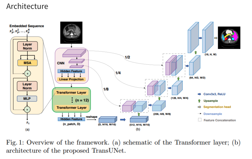
TransUNet - Transformer를 적용한 Segmentation Model 논문 리뷰

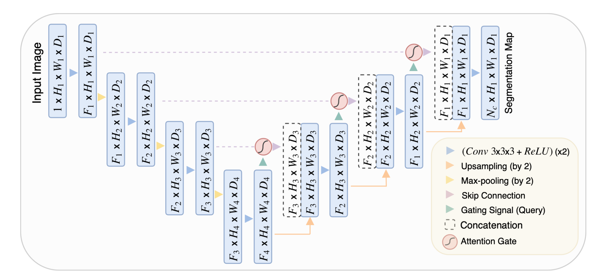
2. Attention U-Net: Learning Where to Look for the Pancreas” by Ozan Oktay et al. (2018)

Attention U-Net: Learning Where to Look for the Pancreas

구현

1. Attention U-Net: Learning Where to Look for the Pancreas” by Ozan Oktay et al. (2018)

Untitled

핵심 코드

   def Attention_U_Net(nClasses, input_height=256, input_width=256, n_filters=16, dropout=0.1, batchnorm=True, n_channels=10):
       inputs = Input(shape=(input_height, input_width, n_channels))
   
       # Contracting Path
       c1 = conv2d_block(inputs, n_filters * 1, kernel_size=3, batchnorm=batchnorm)
       p1 = MaxPooling2D((2, 2))(c1)
       p1 = Dropout(dropout)(p1)
   
       c2 = conv2d_block(p1, n_filters * 2, kernel_size=3, batchnorm=batchnorm)
       p2 = MaxPooling2D((2, 2))(c2)
       p2 = Dropout(dropout)(p2)
   
       c3 = conv2d_block(p2, n_filters * 4, kernel_size=3, batchnorm=batchnorm)
       p3 = MaxPooling2D((2, 2))(c3)
       p3 = Dropout(dropout)(p3)
   
       c4 = conv2d_block(p3, n_filters * 8, kernel_size=3, batchnorm=batchnorm)
       p4 = MaxPooling2D((2, 2))(c4)
       p4 = Dropout(dropout)(p4)
   
       # Bottleneck
       bn = conv2d_block(p4, n_filters * 16, kernel_size=3, batchnorm=batchnorm)
       
       # Expansive Path
       u6 = Conv2DTranspose(n_filters * 8, (3, 3), strides=(2, 2), padding='same')(bn)
       c4 = attention_gate(u6, c4, n_filters * 8)
       u6 = Concatenate()([u6, c4])
       u6 = Dropout(dropout)(u6)
       c6 = conv2d_block(u6, n_filters * 8, kernel_size=3, batchnorm=batchnorm)
   
       u7 = Conv2DTranspose(n_filters * 4, (3, 3), strides=(2, 2), padding='same')(c6)
       c3 = attention_gate(u7, c3, n_filters * 4)
       u7 = Concatenate()([u7, c3])
       u7 = Dropout(dropout)(u7)
       c7 = conv2d_block(u7, n_filters * 4, kernel_size=3, batchnorm=batchnorm)
   
       u8 = Conv2DTranspose(n_filters * 2, (3, 3), strides=(2, 2), padding='same')(c7)
       c2 = attention_gate(u8, c2, n_filters * 2)
       u8 = Concatenate()([u8, c2])
       u8 = Dropout(dropout)(u8)
       c8 = conv2d_block(u8, n_filters * 2, kernel_size=3, batchnorm=batchnorm)
   
       u9 = Conv2DTranspose(n_filters * 1, (3, 3), strides=(2, 2), padding='same')(c8)
       c1 = attention_gate(u9, c1, n_filters * 1)
       u9 = Concatenate()([u9, c1])
       u9 = Dropout(dropout)(u9)
       c9 = conv2d_block(u9, n_filters * 1, kernel_size=3, batchnorm=batchnorm)
   
       # Output Layer
       output = Conv2D(nClasses, (1, 1), activation='sigmoid')(c9)

attention과 unet 자체가 가벼움 각 depth 마다 attention layer가 추가되어 개별적인 추론에 능숙

최고 성능 : 74%

2. 3D TransUNet: Advancing Medical Image Segmentation through Vision Transformers

Untitled

핵심 코드

   def transunet(nClasses, input_height=256, input_width=256, n_filters = 16, dropout = 0.1, batchnorm = True, n_channels=10):
       input_img = Input(shape=(input_height,input_width, n_channels))
   
       # contracting path
       c1 = conv2d_block(input_img, n_filters=n_filters*1, kernel_size=3, batchnorm=batchnorm)
       p1 = MaxPooling2D((2, 2)) (c1)
       p1 = Dropout(dropout)(p1)
   
       c2 = conv2d_block(p1, n_filters=n_filters*2, kernel_size=3, batchnorm=batchnorm)
       p2 = MaxPooling2D((2, 2)) (c2)
       p2 = Dropout(dropout)(p2)
   
       c3 = conv2d_block(p2, n_filters=n_filters*4, kernel_size=3, batchnorm=batchnorm)
       p3 = MaxPooling2D((2, 2)) (c3)
       p3 = Dropout(dropout)(p3)
   
       c4 = conv2d_block(p3, n_filters=n_filters*8, kernel_size=3, batchnorm=batchnorm)
       p4 = MaxPooling2D(pool_size=(2, 2)) (c4)
       p4 = Dropout(dropout)(p4)
   
       # Prepare for Transformer
       p3_flat = Reshape((16*16, 128))(p4)
   
       # Initialize the input for the first Transformer block
       transformer_input = p3_flat
       
           # Create a series of Transformer blocks
       for i in range(4):  # 12 Transformer blocks
           transformer_block = TransformerEncoder(
               filters=n_filters * 8, num_heads=n_filters * 8, ff_dim=n_filters * 8, rate=dropout, name=f"transformer_encoder_{i}"
           )
           transformer_output = transformer_block(transformer_input)
           transformer_input = transformer_output  # Output of the current block is the input for the next
       
       # Reshape back to the spatial dimensions for convolution
       t_encoded_reshaped = Reshape((input_height // 16, input_width // 16, n_filters * 8))(transformer_output)
       
       # expansive path
       u6 = Conv2DTranspose(n_filters*8, (3, 3), strides=(2, 2), padding='same') (t_encoded_reshaped)
       u6 = concatenate([u6, c4])
       u6 = Dropout(dropout)(u6)
       c6 = conv2d_block(u6, n_filters=n_filters*8, kernel_size=3, batchnorm=batchnorm)
   
       u7 = Conv2DTranspose(n_filters*4, (3, 3), strides=(2, 2), padding='same') (c6)
       u7 = concatenate([u7, c3])
       u7 = Dropout(dropout)(u7)
       c7 = conv2d_block(u7, n_filters=n_filters*4, kernel_size=3, batchnorm=batchnorm)
   
       u8 = Conv2DTranspose(n_filters*2, (3, 3), strides=(2, 2), padding='same') (c7)
       u8 = concatenate([u8, c2])
       u8 = Dropout(dropout)(u8)
       c8 = conv2d_block(u8, n_filters=n_filters*2, kernel_size=3, batchnorm=batchnorm)
   
       u9 = Conv2DTranspose(n_filters*1, (3, 3), strides=(2, 2), padding='same') (c8)
       u9 = concatenate([u9, c1], axis=3)
       u9 = Dropout(dropout)(u9)
       c9 = conv2d_block(u9, n_filters=n_filters*1, kernel_size=3, batchnorm=batchnorm)
       
       outputs = Conv2D(1, (1, 1), activation='sigmoid') (c9)
       model = Model(inputs=[input_img], outputs=[outputs])
       return model

transformer가 무거움, 전반적인 구조와 특징을 잘잡음

최고 성능 : 86%

Loss

Combination Loss: Dice and Cross-Entropy Loss

조합: Dice 손실과 크로스 엔트로피(Cross-Entropy) 손실의 조합입니다.
목적: Dice 손실은 예측 마스크와 실제 마스크 간의 유사도를 최대화하는 반면, 크로스 엔트로피 손실은 예측된 확률 분포와 실제 레이블 간의 차이를 최소화합니다. 이 두 손실을 조합함으로써, 모델은 마스크의 형태를 잘 캡처하면서도 개별 픽셀 분류에 대한 성능을 향상시킬 수 있습니다.

Combination Loss: Focal and Tversky Loss

조합: Focal 손실과 Tversky 손실의 조합입니다.
목적: Focal 손실은 잘못 분류된 예측에 더 많은 주의를 기울이고, Tversky 손실은 클래스 불균형과 False Positives 및 False Negatives 사이의 균형을 조절합니다. 이 조합을 사용함으로써, 모델은 클래스 불균형이 심각한 세그멘테이션 문제에서 더 나은 성능을 보일 수 있습니다.

데이터 셋 특징

6번 7번 channel에서 특이점 발견

Untitled

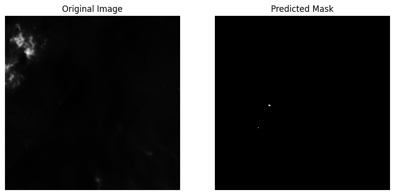
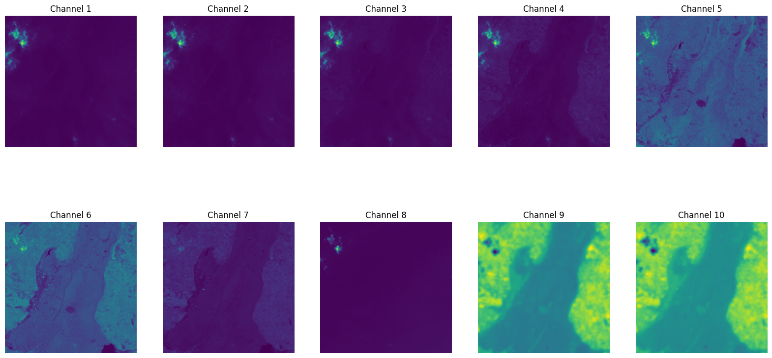
두 그래프를 보면 예측된 값에 이미지랑 겹치는 부분이 6번과 7번에서 밝게 보임

실제 특징을 잡을 수 있는 layer 추가하는 아이디

Segmentation task에서 활용할 수 있는 다양한 Loss

1. Cross-Entropy Loss (Categorical Crossentropy)

If your segmentation task is multi-class where each pixel is classified into one of several categories, categorical crossentropy is a common starting point. It measures the performance of a classification model whose output is a probability value between 0 and 1.

2. Dice Loss

Particularly popular for medical image segmentation and applicable to satellite imagery as well, the Dice loss function is excellent for dealing with class imbalance, which is common in segmentation tasks. It is defined as 1−prediction+truth2∗intersection, effectively measuring how well the predicted segmentation matches the ground truth. Sometimes, it’s combined with cross-entropy loss to leverage the benefits of both.

  import tensorflow as tf
    
  def dice_loss(y_true, y_pred, smooth=1e-6):
      """
      Dice loss, used for imbalanced data.
      :param y_true: True labels.
      :param y_pred: Predictions.
      :param smooth: Small number to avoid division by zero.
      :return: Dice loss.
      """
      # Flatten the labels and predictions
      y_true_f = tf.reshape(y_true, [-1])
      y_pred_f = tf.reshape(y_pred, [-1])
        
      # Calculate intersection and union
      intersection = tf.reduce_sum(y_true_f * y_pred_f)
      union = tf.reduce_sum(y_true_f) + tf.reduce_sum(y_pred_f)
        
      # Calculate the Dice score and then the Dice loss
      dice = (2. * intersection + smooth) / (union + smooth)
      dice_loss = 1 - dice
        
      return dice_loss
    

3. Jaccard Loss (IoU - Intersection over Union)

Similar to Dice loss, Jaccard loss (or IoU loss) is useful for segmentation tasks. It measures the size of the intersection divided by the size of the union of the predicted and ground truth masks. Like Dice, it is robust to class imbalance.

4. Focal Tversky Loss

An extension of the Tversky loss that incorporates the focal loss principle to focus learning more on hard examples and less on easy ones. This can be particularly useful if your model struggles with certain classes or specific areas within the satellite images.

5. Weighted Cross-Entropy Loss

For tasks with significant class imbalance, weighted cross-entropy can provide a mechanism to assign more importance to less frequent classes, ensuring the model doesn’t become biased toward the dominant class.

6. Combined Loss Functions

Often, a combination of the above loss functions (e.g., a weighted sum of Dice loss and cross-entropy loss) is used to leverage the benefits of each. This approach allows you to balance the spatial consistency enforced by Dice or IoU with the pixel-wise classification accuracy of cross-entropy.

몇가지를 조합해서 사용

requirements.txt

numpy pandas rasterio tensorflow==2.14.0 scikit-learn matplotlib keras tqdm joblib opencv-python scipy tifffile jupyter tensorflow-model-optimization

Twitter Facebook LinkedIn

Jongha Kim

[프로젝트] AI Spark 글로벌 산불감지 챌린지, TransUNet, Attention U-Net

Review

약 3주 간에 기록 (24/3/8 ~ 24/3/25)

이전 대회 다른 블로그

참고한 논문 [2가지]

1. 3D TransUNet: Advancing Medical Image Segmentation through Vision Transformers

2. Attention U-Net: Learning Where to Look for the Pancreas” by Ozan Oktay et al. (2018)

구현

1. Attention U-Net: Learning Where to Look for the Pancreas” by Ozan Oktay et al. (2018)

2. 3D TransUNet: Advancing Medical Image Segmentation through Vision Transformers

Loss

Combination Loss: Dice and Cross-Entropy Loss

Combination Loss: Focal and Tversky Loss

데이터 셋 특징

Segmentation task에서 활용할 수 있는 다양한 Loss

1. Cross-Entropy Loss (Categorical Crossentropy)

2. Dice Loss

3. Jaccard Loss (IoU - Intersection over Union)

4. Focal Tversky Loss

5. Weighted Cross-Entropy Loss

6. Combined Loss Functions

requirements.txt

공유하기

참고

[논문분석] A Survey of Large Language Models

[논문분석] DiffTalk: Crafting Diffusion Models for Generalized Audio-Driven Portraits Animation

[논문분석] KAN: Kolmogorov–Arnold Networks

[논문분석] Elucidating the Design Space of Diffusion-Based Generative Models