[논문분석] Video DIffuison Models
Diffusion model의 Video generation, base 논문
[Home, Paper]
Author: Google Research, Brain Team
Abstract
이 모델은 표준 이미지 확산 아키텍처를 자연스럽게 확장한 것으로, 이미지와 동영상 데이터에서 공동으로 학습할 수 있어 미니배치 그라데이션의 편차를 줄이고 최적화 속도를 높일 수 있음.
더 길고 더 높은 해상도의 비디오를 생성하기 위해 이전에 제안된 방법보다 더 나은 성능을 보이는 공간 및 시간 비디오 확장을 위한 새로운 조건부 샘플링 기법을 도입
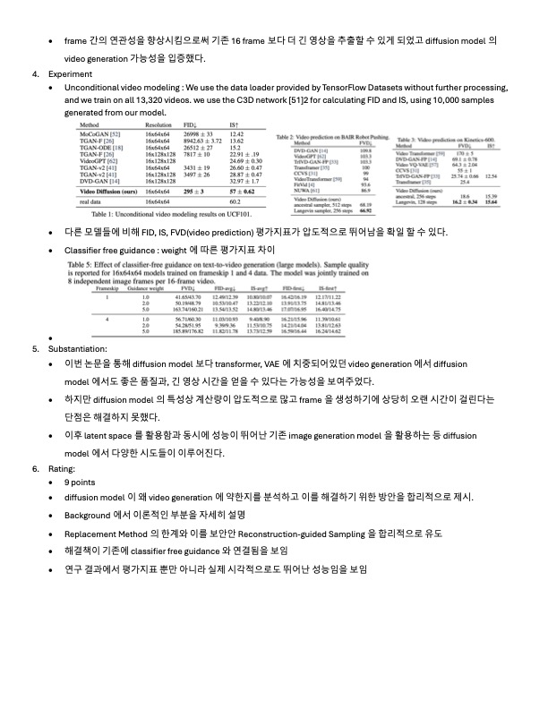
대규모 텍스트 조건부 비디오 생성 작업에 대한 첫 번째 결과와 비디오 예측 및 무조건 비디오 생성에 대한 기존 벤치마크에 대한 최신 결과를 제시
Background
\[q(z_t|\mathbf{x}) = \mathcal{N}(z_t; \alpha_t\mathbf{x}, \sigma_t^2I) \rightarrow q(z_t|z_s) = \mathcal{N}(z_t; \frac{\alpha_t}{\alpha_s}z_s, \sigma^2 I)\]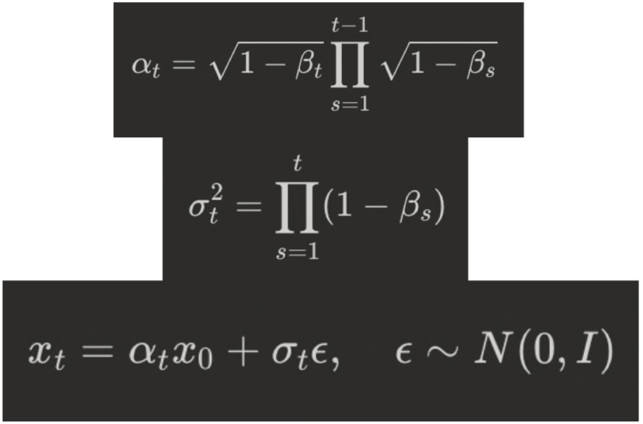
왼쪽 조건식을 통해 아래 평균과 분산을 구한다.
\[x_t = \alpha x_0 + \sigma_t \epsilon\]다음 식의 경우 변형된 식을 Training 에서 사용
\[\widehat{\mathbf{x}}_\theta(\mathbf{z}_t) = {\mathbf{z}_t-\sigma_t\epsilon_\theta(\mathbf{z}_t)\over \alpha_t}\]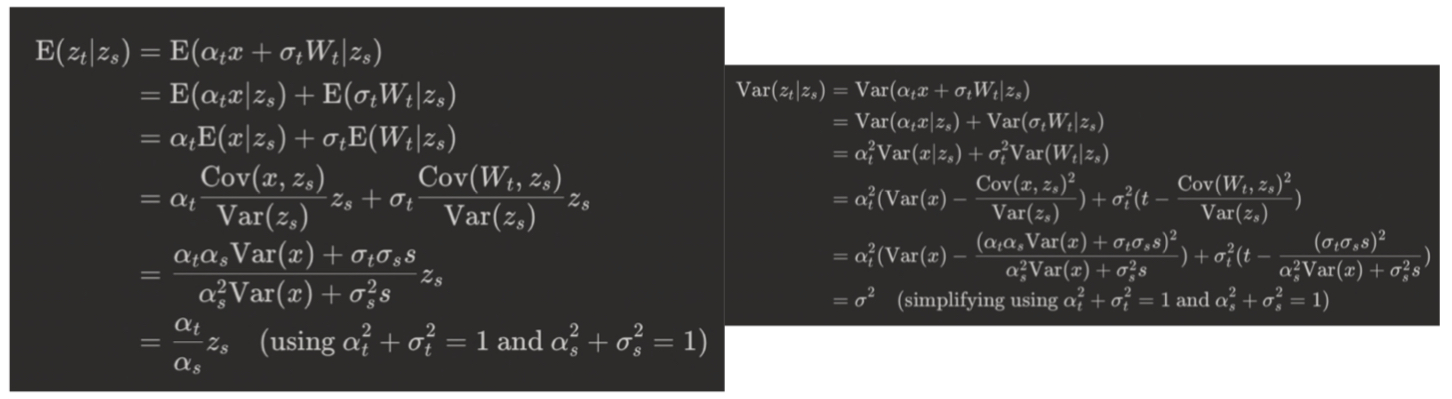
Training
forward process를 역으로 학습
\[E_{ε,t} [w(λ_t) \parallel \widehat{\mathbf{x}}_θ(\mathbf{z}_t) − \mathbf{x} \parallel^2_2]\]가중 MSE loss를 사용하여 denoising model \(\hat{x}_
θ\)
를 학습
variational lower bound
ϵ-prediction parameterization
\[\widehat{\mathbf{x}}_\theta(\mathbf{z}_t) = {\mathbf{z}_t-\sigma_t\epsilon_\theta(\mathbf{z}_t)\over \alpha_t}\]이때 \(\epsilon_\theta(\mathbf{z}_t)\) 는 다음과 같이 정의
PDF의 미분꼴
-
V-prediction parameterization
Denoising Diffusion Probabilistic Models (DDPM) 과 관련된 기술로 노이즈를 예측하는 방법
V-prediction 파라미터화는 이러한 복원 과정에서 ‘노이즈를 직접적으로 예측하는 방식’과는 다른, 대안적인 방식 (일반적으로는 epsilon 예측 (ε-prediction) 방식이 사용)
\[v_t = \sqrt{\frac{\alpha_t}{1-\alpha_t}} x_0 + \sqrt{\frac{1-\alpha_t}{\alpha_t}} \epsilon_t\]Vt는 노이즈와 원본 데이터의 혼합물로, 모델은 이 Vt를 예측
시간에 대한 의존성 줄이기 → 각 시간 단계에서 독립적으로 작동 → 병렬처리 효율적인 계산
Sampling
- ancestral samplier
sampling variances derived from lower and upper bounds on reverse process entropy
\[q(\mathbf{z}_s|\mathbf{z}_t,\mathbf{x}) = N(\mathbf{z}_s;\tilde{μ}_{s|t}(\mathbf{z}_t,x),\tilde{σ}^2_{s|t} I)\] \[\tilde{μ}_{s|t}(\mathbf{z} ,\mathbf{x})=e^{λ_t−λ_s}(α_s/α_t )\mathbf{z}_t +(1−e^{λ_t−λ_s})α_s \mathbf{x}\quad and \quad \tilde{μ}_{s|t}^2 =(1−e{λ_t−λ_s})σ_s^2\]so
\[\mathbf{z}_s =\tilde{μ}_{s|t}(\mathbf{z}_t,\widehat{\mathbf{x}}_θ(\mathbf{z}_t))+\sqrt{(\tilde{σ}_{s|t}^ 2 )^{1−γ}(σ_{s|t}^2 )γε}\]- the predictor-corrector sampler
Our version of this sampler alternates between the ancestral sampler step and a Langevin correction step (효과적)
\[\mathbf{z}_s←\mathbf{z}_s−{1\over2}δσ_sε_θ(\mathbf{z}_s)+ \sqrt{δ}σ_sε^\prime\]δ : step size (fixed 0.1 in paper)
\(ε^\prime\) : independent sample of standard Gaussian noise
Langevin 은 각 step의 marginal distribution(주변 분포) \(\mathbf{z}_s$가 $\mathbf{x}\sim P(\mathbf{x})\) 에서 부터 시작된 true한 marginal distribution이 될 수 있게함
- classifier-free guidance
\(w\) : guidance strength
\[ε_θ(\mathbf{z}_t, \mathbf{c}) = {1\over\sigma_t} (\mathbf{z}_t − \hat{\mathbf{x}}_θ(\mathbf{z}_t, \mathbf{c}))\]: the regular conditional model prediction
Video Diffusion Models
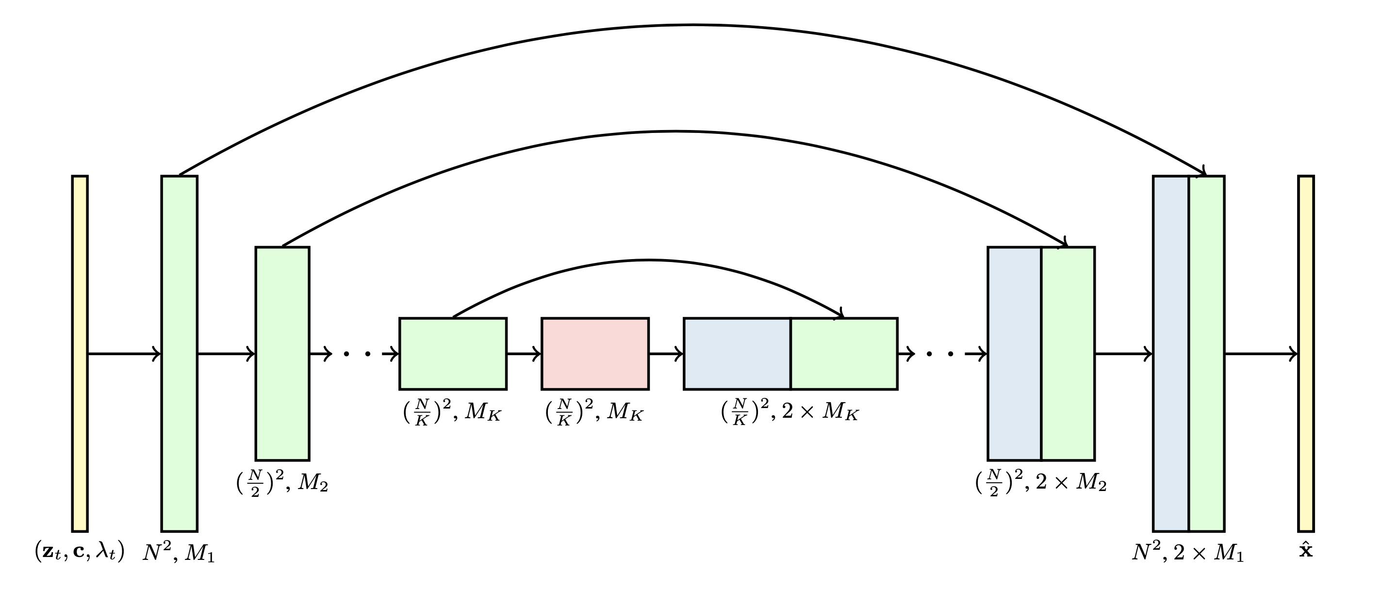
3D U-Net architecture
3D U-Net architecture를 활용해서 reverse process를 구현 (denoising score matching 방법으로 학습)
기존에 image diffusion model architecture 에서 video data로 확장하기 위해 3D U-Net을 활용
Fixed number of frame 출력
3D U-Net 을 사용하지만 3D를 직접적으로 사용하는 것은 아님. 1 x 3 x 3 의 convolution을 사용 한다. (temporal domain x hight x width)
skip connection 사용
spatial attention block → temporal attention block (각각 독립적으로 존재하며 순차적으로 진행)
Each block represents a 4D tensor with axes labeled as frames × height × width × channels
이때 channel은 입력 데이터의 특징을 담으며, channel 수가 많을 수록 특징을 더 잘 잡지만, 메모리가 증가한다.
→ image generation ,video generation 동시에 학습
Reconstruction-guided sampling for improved conditional generation
| 16개 초기 이미지 frame 이후에 추가적인 프레임 생산 → $$\mathbf{x}^b \sim p_\theta(\mathbf{x}^b | \mathbf{x}^a)$$ |
(memory 한계로 인해 한번에 16개 밖에 못 만듦)
-
autoregressive (\(\mathbf{x}^a \sim p_\theta(\mathbf{x})\) → $$\mathbf{x}^b \sim p_\theta(\mathbf{\mathbf{x}^b \mathbf{x}^a})$$) : conditional diffusion 을 활용, 16개 프레임 이후에 나올 frame 예측 - imputation : 초기 frame 간격 사이에 들어갈 frame 예측
- super resolution
| 1,2 번 두 접근 방식 모두 조건부 모델 $$p_θ(x^b | x^a)$$에서 샘플링 + 별도로 학습된 모델이 필요하지 않다는 이점 |
Replacement Method
Score-based generative modeling through stochastic differential equations 논문
conditional sampling : 어떤 비디오 프레임 xa가 주어졌을 때 다른 프레임 xb의 분포를 추정하는 것입니다. 예를 들어, xa가 비디오의 첫 번째 프레임이고 xb가 두 번째 프레임이라면, 조건부 샘플링은 xa와 일관성 있는 xb를 생성하는 것입니다.
diffusion model 을 다음 식을 통해 학습 , \(p_\theta(\mathbf{x} = [\mathbf{x}^b,\mathbf{x}^a])\)
이때 \(x^a\) 의 noise 버전인, \(z^a_s\) 를 정확하게 계산하여 reverse process에 입력으로 교체되기 때문에 replacement method
-
$$p_\theta(\mathbf{x}^b \mathbf{x}^a)$$ 활용 빠르고 정확한 sampling, 하지만 조건부 모델을 따로 학습해야함
\(\mathbf{x}^a\) 고정 ,\(z^a_s\) 를 계산 후 \(\mathbf{x}^b\) 와 함께 2개의 입력을 노이즈로부터 reverse process를 통해 생성
-
\(p_\theta(\mathbf{x})\) 활용
\(\mathbf{x}^b , \mathbf{x}^a\) 를 하나의 벡터 x로 결합하고 unconditional model을 통해 x를 재구성
하나의 모델로 여러 conditional sampling진행 가능, 하지만 느리고 부정확 할 수 있음
\(\mathbf{x}^a, \mathbf{x}^b\) 로 부터 \(z^a_s, z^b_s\) 를 동시에 계산 후 reverse process를 거침
더 정확한 조건부, 하지만 복잡한 계산
but, 이 방법은 video generation에 적합하지 않음
문제점 : xb의 노이즈 버전 zbs가 xa와 무관하게 업데이트된다는 것
\[x^b_θ(z_t)=x^b_θ(z_t)− {α_t^2\over 2}∇_{z^b_t}{logq(x^a|z_t)}\]다음 식을 보면 두번째 항이 사라짐
생성된 frame이 초기 frame 부분과의 일관성이 떨어짐
score function(denoisier)이 U-Net으로 설정되어있어 foward pass와 implicit하게 학습하기 힘듬
이를 해결하는 방법으로 각 iteration마다 fowardpass 에서 처럼 noise를 더하는 과정을 추가
이방법은 computationaly heavy
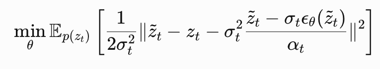
Gradient Method (novelty)
reconstruction-guided sampling
이는 guidance항을 추가한 형태로 reconstruction-guided sampling 또는 단순히 reconstruction guidance라 부른다.
\[x^b_θ(z_t)=x^b_θ(z_t)− {w_rα_t\over 2}∇_{z^b_t}{∥x^a−x^a_θ(z_t)∥}^2_2\]다음과 같이 변형하여 사용
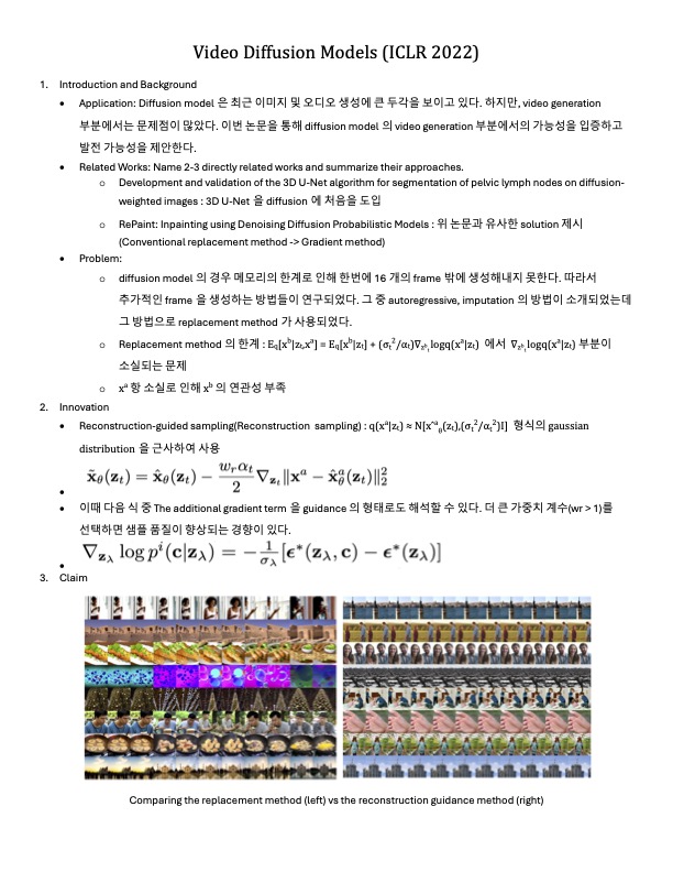
Experiments
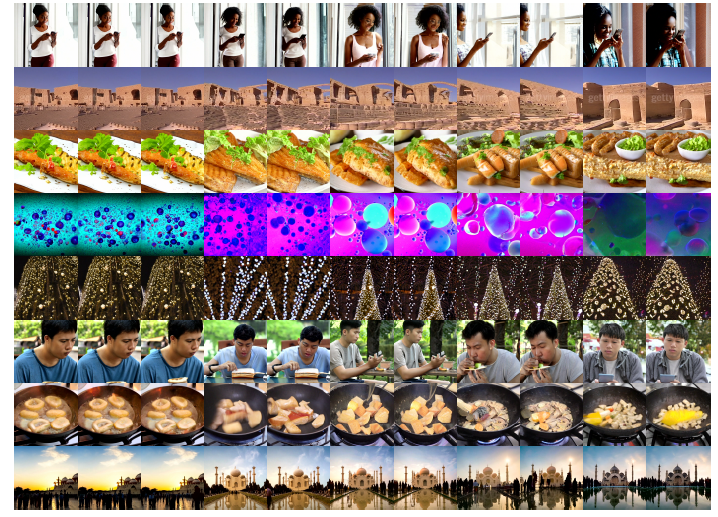
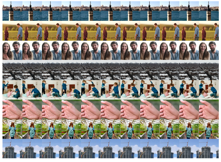
replacement 방법(왼쪽)과 reconstruction guidance 방법(오른쪽)
Summary